Modelling Car Suspension with ODE's: Damped Free Oscillations Part 2

masterwu (59)in #steemstem • 6 years ago (edited)

In the mathematical modelling of the mass-damper-spring system (Figure 1), we've explored the underdamped case in the previous post.

Figure 1. Schematic of the mass-damper-spring system (adapted from Wikimedia Commons)

We seen that with an under damped suspension system (case I), a car can wallow up and down whenever it goes over a speed bump, making it very difficult for the driver to control the vehicle.

Before we explore the case II, critical damping, let's recap the equation of motion for the mass-damper-spring system...

where:

= sprung mass [kg]
= damping coefficient [Ns/m]
= spring constant [N/m]

...we can have 3 different cases...

Case I	< 0	Under damping
Case II	= 0	Critical damping
Case III	> 0	Over damping

Case II: Critically Damped

Critical damping is the border case between oscillatory (under damped) and non-oscillatory (over damped) motions.

Let's take explore our car suspension model with the damper tuned to be critically damped. The parameters from the previous post...

sprung mass m = 300kg
spring constant k = 1200N/m
initial displacement = 0.15m
initial velocity = 0m/s

The system is critically damped when...

Substituting above parameters, we need to tune the damper to...

A diagram of the system is shown in Figure 2 below...

Figure 2. Suspension schematic with parameters required for critical damping

Now that we have the damping coefficient for the critically damped case, substituting these into equation (1), the equation of motion becomes...

The characteristic equation of (2)...

The only root of equation (3) is...

Now according to equation (8) of Post #3, the general solution is...

Applying the first initial condition (initial displacement)...

The first derivative of the general solution, equation (4) is...

Now we can apply the second initial condition (initial velocity)...

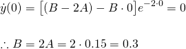
Therefore, the particular solution is...

The behaviour of the particular solution is shown in Figure 3...

Figure 3. Behaviour of the suspension system with and

As you can see, the car pretty much returns to its equilibrium position in less than 4 seconds, which is quite a slow response for most real-world applications.

Exploring the initial value problem

Let's now explore the solution with a few different permutations for the initial conditions...

initial displacement = 0.15m, therefore A = 0.15
initial velocity = -0.6m/s

Substituting this values into equation (5)...

This gives rise to the particular solution is...

What about the following?...

initial displacement = 0.15m, therefore A = 0.15
initial velocity = -0.3m/s

This gives rise to the particular solution...

And the following permutation...

initial displacement = 0.15m, therefore A = 0.15
initial velocity = 0.3m/s

...gives rise to the particular solution...

All of the above solutions are superimposed in Figure 4...

Figure 4. Various particular solutions to the critically damped car suspension problem.

Finally, let's see how the suspension behaves with zero initial displacement, but a non-zero initial velocity. For instance...

initial displacement = 0.0m, therefore A = 0.0
initial velocity = 0.3m/s

Again, from equation (5), we have...

...giving rise to the particular solution...

A few solutions showing the behaviour of the mechanism with varying values of ...

Figure 5. Various particular solutions to the critically damped car suspension problem.

Discussion about the above case...

Critical damping is what car manufacturers aim for in most cases. As we have seen with under damping, the residual vibrations that occur after hitting a bump can be very dangerous in terms of steering and car control. It can also cause passengers who are susceptible to motion sickness to become ill.

With over damping, which we will explore in the next post, the shock absorber is stiff and sluggish, which means it is slow to respond to bumps. This means that bumps are not absorbed as much and car returns to its equilibrium position slowly, making the ride quite uncomfortable. It feels like a car with no suspension, and may compromise the car's grip on rougher roads, because the wheels are in less contact with the ground at certain times (the car might do a "jump" when it hits a bump).

As I have mentioned previously, the parameters used for the this particular suspension set up is quite "soft" and "squishy" for most real-world applications. We have a soft spring at 1200N/m, and the critical damping coefficient for this softly sprung car will dissipate a bump of 15cm in about 4 seconds.

Credits:

All equations in this tutorial were created with QuickLatex

All graphs were created with www.desmos.com/calculator