Modelling Car Suspension with ODE's: Damped Free Oscillations Part 1

masterwu (59)in #steemstem • 6 years ago (edited)

In my previous post, I stated that all real world free oscillating systems are damped because their vibrations eventually attenuate away, due to energy dissipation to the surrounding environment.

However, for many engineering applications, the natural damping may not be enough. One way to damp oscillations quicker is to have the vibrating mass move through a viscous fluid, thus the energy of the motion is dissipated as heat through the thick fluid (as it causes the fluid to move).

Indeed, many real-life engineering applications use the concept of viscous damping, such as shock absorbers on mountain bike, motor cycle and car suspension systems.

Figure 1. Rear suspension on a historic Lotus Formula 1 car.
Source: Wikimedia Commons

In Figure 1, we can see that the engineers have coiled the spring over a shock absorber which is filled with oil. This is a common arrangement in many modern cars to make mounting this type of suspension easier.

A schematic of a mass-spring mechanism undergoing viscous damping is shown in Figure 2...

Figure 2. Schematic of the mass-spring-damper system. Adapted from Calculus 5th Edition, James Stewart.

Like the spring, the damping force is always opposing the motion of the mass. A good approximation (confirmed by physical experiments) is the damping force is linearly proportional to the velocity of the mass, hence .

Thus with a damped system, the mass now has 2 opposing forces. Firstly...

And secondly...

These forces are shown in blue, in Figure 2. Again, by Newton's 2nd Law, the resultant force on an object is equal to its mass by its acceleration...

Expressing acceleration as the second time derivative of displacement, we can rearrange equation (1) into a Second Order, homogeneous, linear ODE with constant coefficients...

The characteristic equation of (2) is...

...and the roots of (3) are...

Now let the discriminant Δ equal the term inside the square-root and we have the same situation as that of Post #3 in this series: Roots of Homogeneous Second Order ODE's and the Nature their Solutions, where the behaviour of the solution will depend on the value of Δ.

So with...

...we can have 3 different cases...

Case I	< 0	Under damping
Case II	= 0	Critical damping
Case III	> 0	Over damping

Case I: Under damping

Suppose that we are investigating the suitability of a new car suspension system. If we focus our attention on just one corner of the car, we can simplify the suspension to our mathematical mass-spring-damper model.

Let's assign the system system with the following parameters...

mass m = 300kg (total car body mass of 1200kg)
spring constant k = 1200N/m (note, this is a very soft spring compared to real world applications)
damping constant c = 600Ns/m
initial displacement = 0.15m (let's say this wheel has been driven off a curb of 15cm height, and therefore the spring is stretched by this amount as our starting position)
initial velocity = 0m/s

A schematic of this system is shown in Figure 3 below...

Figure 3. Schematic of a simplified car suspension
(adapted from Wikimedia Commons)

Substituting this values for m, c and k in to equation (2), we have...

Characteristic equation for (4) is...

The roots of (5) are...

As we have complex conjugate roots, the general solution to equation (4), according equation (11) of Post #3 is...

Let's find the particular solution of (6) by applying the initial conditions. First, applying the initial displacement condition...

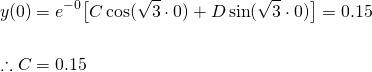
The first derivative of (6) is...

Now we can apply the initial velocity to equation (7)...

Therefore, the particular solution is...

The "amplitude phase-shift" equivalent solution is...

The behaviour of the solution of equation (9) shown in Figure 3 below...

Figure 3. Free oscillations with damping coefficient c = 600Ns/m

As you can see, the motion attenuates quickly after 2 oscillations (including the initial displacement), with the peak of the second oscillation a mere fraction of the amplitude of the first. Note, although the oscillations are damped out quickly, this is still a case of under damping according to the mathematics.

So what happens when we lower the damping coefficient (or tune the damper down) to say, c = 150Ns/m?

Equation (2) becomes...

And the characteristic equation for (10) is...

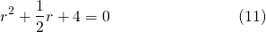
The roots of (11) are...

As previously, from these roots, the general solution is...

And as previously, applying both initial conditions, the particular solution is...

The "amplitude phase-shift" equivalent solution...

The behaviour of (14) shown in Figure 4 below...

Figure 4. Free oscillations with damping coefficient c = 150Ns/m

Now there are at least 6 oscillations before the motion peters out. Do you think this is a good performance from a car's suspension? This car's going to bump up and down 6 times with every pothole it drives over!

Take a look at the video below (published by Open University) which excellently explains what happens to a car when it is severely underdamped. Enjoy.