Introduction to Second Order Differential Equations

Let's take a dive into the fascinating world of Second Order Differential equations. These have very important applications in engineering, and you'll see them repeatedly in the modelling of electrical signals and mechanical vibrations.

Figure 1. Chladni's Experiment. Pattern formed by sand in response to the vibration of the plate it is placed on.
Image source: Wikimedia Commons

Generally, a homogeneous, linear, Second Order Differential equation has the form...

...where y(x) is a (at least) twice differentiable, unknown function on any open interval.

Equation (1) homogeneous by virtue of the equation equalling 0. If the right hand side of the equation was a non-zero function (including constants), then the equation would be considered non-homogeneous.

Equation (1) has an infinite number of solutions, which can be expressed in the form of a general solution.

But more pertinently, the general solution should be expressed as a linear combination of all linearly independent solutions. I know that sounds like gibberish, so let me explain...

For example...

For equation (1), if we make the functions P(x) and R(x) equal to 1, and the function Q(x) equal to 0, then we have...

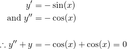
You might notice that a possible solution to equation (2) is y = cos(x), since...

But equally, y = sin(x) is also a possible solution as you can verify for yourself. Therefore, if we add the two solutions, we can still satisfy equation (2).

Thus...

...is also a solution of (2). This is called the principle of superposition.

But, we can be more general still, because multiples of cos(x) and sin(x) can also be solutions. So the most general form of the solution to equation (2) is...

...where A and B are arbitrary constants.

Now, and are linearly independent functions because one cannot be expressed as a constant multiple of another, or in other words, they are not proportional to each other.

Finding solutions

It's generally not that easy to find particular solutions to equation (1). A lot of times, we'll have to resort to complex, creative analytical methods. Sometimes, we'll require numerical methods to approximate solutions.

For now, let's focus on simpler equations that we can solve. If we let P(x) = a, Q(x) = b and R(x) = c such that they're all constants, then equation (1) becomes...

In all of my posts on First-Order, linear differential equations, all solutions involved an exponential function. So it's reasonable to assume that an exponential function would for the basis for the solutions to Second-Order equations as well.

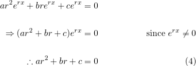
So let's try , because the second and first derivative of this function are constant multiples of itself. So substituting this into equation (3), we get...

Equation (4) is called the characteristic equation or the auxiliary equation. Being a quadratic equation, we can find the roots using the quadratic formula...

...and thus possible solutions to equation (3) are and

Using the principle of superposition, the general solution for equation (3) is...

Particular solutions

Inasmuch as the particular solution to a First Order Differential equation relies on having to satisfy an initial condition, the particular solution to a Second Order Differential equation relies on satisfying 2 initial conditions, because we have 2 unknown constants in A and B.

Say the initial conditions are...

Applying these initial conditions to equation (5), we get...

Solving equations (6) and (7), we get the particular solution...

So we've derived the particular solution of equation (3) mathematically. However, what the limitation of leaving the solution in this form is it is difficult to understand its behavior or its the physical characteristics it is modelling. We'll delve into that on the next post...

---

First Order Differential Equations

1. Introduction to Differential Equations - Part 1
2. Differential Equations: Order and Linearity
3. First-Order Differential Equations with Separable Variables - Example 1
4. Separable Differential Equations - Example 2
5. Modelling Exponential Growth of Bacteria with dy/dx = ky
6. Modelling the Decay of Nuclear Medicine with dy/dx = -ky
7. Exponential Decay: The mathematics behind your Camping Torch with dy/dx = -ky
8. Mixing Salt & Water with Separable Differential Equations
9. How Newton's Law of Cooling cools your Champagne
10. The Logistic Model for Population Growth
11. Predicting World Population Growth with the Logistic Model - Part 1
12. Predicting World Population Growth with the Logistic Model - Part 2
13. What's faster? Going up or Coming Down?

First order Non-linear Differential Equations

1. There's a hole in my bucket! Let's turn it into a cool Math problem!
2. The Calculus of Hot Chocolate Pouring!
3. Foxes hunting Bunnies: Population Modelling with the Predator-Prey Equations

Second Order Differential Equations

1. Introduction to Second Order Differential Equations

---

Please give me an Upvote and Resteem if you have found this tutorial helpful.

Please ask me a maths question by commenting below and I will try to help you in future posts.

I would really appreciate any small donation which will help me to help more math students of the world.

Tip me some DogeCoin: A4f3URZSWDoJCkWhVttbR3RjGHRSuLpaP3

Tip me at PayPal: https://paypal.me/MasterWu