Support Vector Regression: All You Need to Know
I was working on Support Vector Regression(SVR) recently and tried to understand the concept behind it. It was very hard for me to find about SVR. Most of the theory was releated to SVM. With continous effort, I end up collecting some information on SVR. I am writing this blog to future user who wants to clear the conept on SVR. Since I am also learning it recently, I might have made some errors. If there are any errors or if I misunderstood anything here, please let me know.
Support Vector Machine(SVM) was first proposed by Vapnik is one of most used and efficient method for classification and regression analysis. SVM is supervised learning method which means target or outcome variable is known beforehand while training the data sets. The main theme of SVM is a construction of a hyperplane that can be used for classification, regression, or other tasks like outliers’ detection.
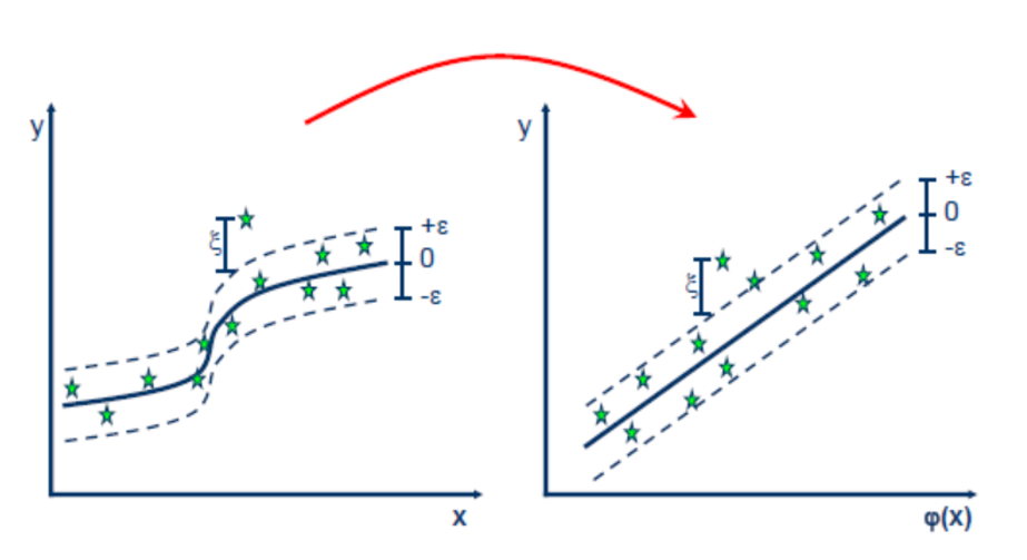
A version of SVM for regression was proposed in 1996 by Vladimir N. Vapnik, Harris Drucker, Christopher J. C. Burges, Linda Kaufman and Alexander J. Smola.[36] This method is called support vector regression (SVR). SVR is very similar to Support Vector Classification but the significant difference is that the cost function in classification doesn’t care the subset of training data which are beyond the margin while the cost function of regression doesn’t care the subset of training data that are closed to model prediction. Instead of margin in classification model, we have a tube in regression. This tube is a ε-insensitive tube which means all the training data points which in the tube don’t contribute any losses. Only the data points outside of the tube contribute the losses.

The SVR problem is like a linear regression problem, unlike a linear line a ε-insensitive tube is fitted in this problem. But in a real-world problem, the training data in feature space are not always linear. Thus, there is need to transform the given feature space into the higher dimensional where the problem becomes linear. Thus, the Kernel function is used to transform the given feature space into higher dimensional space as shown in the figure above.
As it turns out, while solving the SVM, we only need to know the inner product of vectors in the coordinate space. Say, we choose a kernel K and P1 and P2 are two points in the original space. K would map these points to K(P1) and K(P2) in the transformed space. To find the solution using SVMs, we only need to compute inner product of the transformed points K(P1) and K(P2). If S denotes the similarity function in transformed space (as expressed in the terms of the original space), then:
S(P1, P2) = <K(P1),K(P2)>
The Kernel trick essentially is to define S in terms of original space itself without even defining (or in fact, even knowing), what the transformation function K is.
There are different types of kernel functions and most popular of them are enlisted below:
- Linear Kernel: It is given by the inner product of the data in the feature space and is represented as:

- Polynomial Kernel: Polynomial kernels are well suited for problems where all the training data is normalized. It is popular in image processing and represented as:

3.Gaussian or radial basis function (RBF):
It is general-purpose kernel; used when there is no prior knowledge about the data. Equation is:

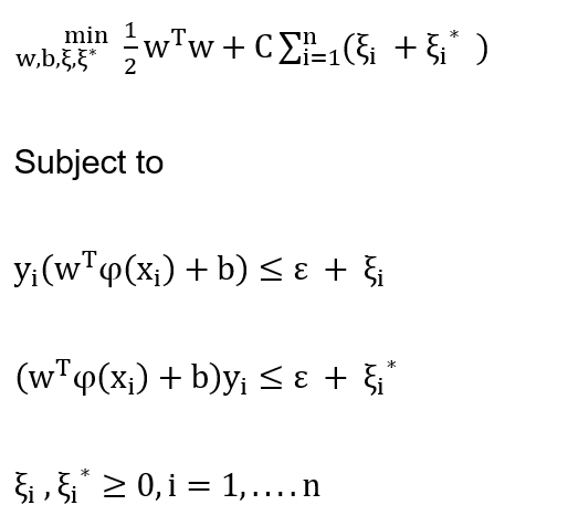
The minimization of the training error in a ε-insensitive tube is like a minimization problem. It is convex optimization problem has one global minima and don’t suffer from local minima. While reducing the error in training data ξ, the problem is prone to overfitting. It tends to memorize the training data and will not do well for the unseen testing data. Because of this, there is need of the term to simplify the model. 1/2 w^T w is the term added to the optimization problem and is called model complexity term.
Now, the support vector regression problem can be represented as a minimization problem as:

where (xi, yi) are a pair of input and output vectors, n is the number of samples, ω is weight factor, b is the threshold value, and C is error cost or a value that controls the penalty imposed on observations that lie outside the epsilon margin (ε) and helps to prevent overfitting (regularization). Input samples are mapped to higher dimensional space by using kernel function φ; ξ is the training error subject to ε-insensitive tube. The ξ and ξ also known as slack variables allow for some data points to stay outside the confidence band determined by ε. The kernel function is responsible for nonlinear mapping between input and feature space. In this formulation, Gaussian kernel the function is used.
I was summoned by @lawlees. I have done their bidding and now I will vanish...
A portion of the proceeds from your bid was used in support of youarehope and tarc.
Abuse Policy
Rules
How to use Sneaky Ninja
How it works
Victim of grumpycat?
You got a 6.91% upvote from @nado.bot courtesy of @lawlees!
Send at least 0.1 SBD to participate in bid and get upvote of 0%-100% with full voting power.
This post has received a 6.10% upvote from @aksdwi thanks to: @lawlees.
You got a 13.97% upvote from @redlambo courtesy of @lawlees! Make sure to use tag #redlambo to be considered for the curation post!
!originalworks