[Steem Analysis] Whaling in the Reps - Looking at SP Versus Reputation
Thar She Blows -- Vast Quantities of Steem
One of the interesting things involved with becoming one of the serious geeks that dig around in the actual content of the blockchain and try understanding what's actually going on under the hood (which I do not advise anyone to do if you want to keep any illusions about your place in the world; always avoid seeing the sausage made) is the lines of conversation that you tend to end up in.
Recently I was talking to someone about Reputation and how it actually operates in practice, not in legend. I was laboring under the misapprehension that Reputation was one of the few places on the blockchain that Steem Power wasn't the end-all be-all of command and control. I thought that it was purely a function of people with higher Reputation voting you up bringing you up or people, in sufficient numbers, voting you down bringing you down.
It turns out that's not the case. It's one more place where SP is the true determinant of how much effect one can have.
That was a disappointing discovery and probably deserves a post all its own, but it led me to another thought.
I wonder what the overlap is between high SP accounts and high Reputation accounts, and how I could best show that relationship.
On a day when the total number of accounts on the steem blockchain has finally exceeded 800k, this is a particularly auspicious time to look at such things.
Let's do that.
Build the Box
As usual, we're going to start by setting up a query for SteamData, because it is truly the easiest way to go digging around in the database without getting a bunch of fields I'm not interested in or other ridiculous mumbo-jumbo. If you haven't seen me do this before, you'll want to look at some of my previous posts for more detail on exactly what's going on. Or ask in the comments. Whatever works for you.
# Setting up the imports for our basic query tools

from steemdata import SteemData
import datetime
from datetime import datetime as dt

import math

import pandas as pd
# Init connection to database

db = SteemData()
Let's just load up our data structure with every account created. It's not that big, right?
We'll be wanting just a few fields from every account: name, reputation, and how many vesting shares that account controls. No more, no less. Everything else we can calculate from that data.
query = {}

proj = {'name': 1,
        'reputation': 1,
        'vesting_shares.amount': 1,
        '_id': 0}

# sort = [('vesting_shares.amount', -1)]
sort = []
result = db.Accounts.find(query,
                          projection=proj,
                          sort=sort)
%%time

Res = list(result)
Wall time: 36.3 s
len(Res)
803516
As expected, just over 800k accounts and a few things about each of them.
Let's bring in the Reputation calculator that we wrote in the last post. The short version is that it takes the total number of vests in log-base-10, then shifts it up by 25. Essentially. This one has been tweaked slightly to take a string or an int and Do The Right Thing(tm) because the database itself stores vests in a mix of ints and strings. Might as well deal with that here and not have to think about it on the feeding side.
def rep2Rep(RawI):
    if isinstance(RawI, int):
        if RawI != 0:
            if RawI > 0:
                return  int(max((math.log( RawI, 10) - 9), 0) * 9) + 25
            else:
                return -int(max((math.log(-RawI, 10) - 9), 0) * 9) + 25
        else:
            # Because we arbitrarily center at 25
            return 25
    else:
        return rep2Rep(int(RawI))
Since we have the data from the database and a computed value that will need to go in alongside, I just go ahead and build a big list of dictionaries, knowing that I'm going to feed it to a pandas DataFrame as soon as I can. Once we get the information into pandas, manipulating it becomes a lot easier, as you'll see.
Result = []

for e in Res:
    Result.append({'name': e['name'],
                  'reputation': int(e['reputation']),
                  'vests': e['vesting_shares']['amount'],
                  'rep': rep2Rep( e['reputation'] )
                  })
ResT = pd.DataFrame(Result)
ResT.head()
| name | rep | reputation | vests | |
|---|---|---|---|---|
| 0 | a-0 | 25 | 0 | 13873.020360 |
| 1 | a-00 | 25 | 0 | 12422.163690 |
| 2 | a-1 | 25 | 0 | 92666.095503 |
| 3 | a-100-great | 25 | 0 | 1027.035201 |
| 4 | a-11 | 44 | 144960973983 | 15412.752588 |
All the data is poured into a single DataFrame, so let's start slicing and dicing it into stuff that we need – in particular, different sortings.
Once we have information in some sort of sorted presentation, we can start making interesting comparisons. We are definitely interested in what sort of thing lives at the top of the Reputation and SP scales, so let's build a couple of versions of this table which are deliberately sorted, one with the highest reputations at the top and the other with the highest vests at the top.
Luckily for us, this is pretty straightforward.
RepT = ResT.sort_values('reputation', ascending=False).set_index('reputation')

RepT.head()
| name | rep | vests | |
|---|---|---|---|
| reputation | |||
| 915099810768682 | steemsports | 78 | 2.338242e+07 |
| 749832145587920 | knozaki2015 | 77 | 1.012949e+08 |
| 688377358041661 | papa-pepper | 77 | 2.866042e+07 |
| 674973077592531 | haejin | 77 | 1.741729e+08 |
| 662798410280792 | gavvet | 77 | 7.260105e+08 |
RepT.tail()
| name | rep | vests | |
|---|---|---|---|
| reputation | |||
| -14045827790498 | r4fken | -12 | 7.235129e+01 |
| -27396614970069 | chainflix | -14 | 3.730789e+05 |
| -29358783062784 | matrixdweller | -15 | 4.698676e+04 |
| -37765258368568 | wang | -16 | 2.851960e+03 |
| -49693494004283 | berniesanders | -17 | 8.749655e+06 |
All of that looks about as we would expect. The top of the list is very clear, holding exactly the people we would expect, as is the bottom.
Let's do the same for vests. There's no need to look at the bottom of the vests list because we know what lives down there, accounts which have been completely vampiricly drained of their SP by another account. Their shambling, dead eyes really worry me, so I'm not going to look.
VesT = ResT.sort_values('vests', ascending=False).set_index('vests')

VesT.head()
| name | rep | reputation | |
|---|---|---|---|
| vests | |||
| 9.003985e+10 | steemit | 35 | 12944616889 |
| 3.385447e+10 | misterdelegation | 25 | 0 |
| 2.124977e+10 | steem | 25 | 0 |
| 1.570402e+10 | freedom | 25 | 0 |
| 9.516259e+09 | blocktrades | 70 | 128868106146117 |
That looks solid.
We can already see something notable right here, in that three of the top five most invested accounts on the blockchain have zero reputation. Specifically zero. If we were looking for accounts which had something strange about them, this would be one of the places to start looking.
We already know that these accounts were created at the origin of the blockchain in prehistory so there's no real need to continue poking at them, but if you wanted to be a junior super sleuth, note that this is the sort of thing that should prick your ears in any other context.
The data is well and truly lined up. Now I want to do something a little strange, and to do that I'm going to need to build a different kind of data structure. This can probably all be done in panda, but I'm a little old school.
First, a list which contains the name of all the accounts and the amount by which they are vested as simple tuples.
VesNL = list(zip(VesT['name'], VesT.index))
VesNL[:5]
[('steemit', 90039851836.6897),
 ('misterdelegation', 33854469950.665653),
 ('steem', 21249773925.079193),
 ('freedom', 15704020549.786041),
 ('blocktrades', 9516258580.957226)]
And now, the same sort of thing except with reputation.
RepNL = list(zip(RepT['name'], RepT['rep']))
RepNL[:5]
[('steemsports', 78),
 ('knozaki2015', 77),
 ('papa-pepper', 77),
 ('haejin', 77),
 ('gavvet', 77)]
Here's where we're going:
Imagine that each of these lists containing 800,000+ accounts, were lying in front of you. Take your left index finger and put it on the first account on the Reputation sheet. Take your right index finger and put it on the first account on the Vests sheet.
Now begin going down the left-hand and right-hand list at the same time. Every time you find a new name under your left index finger, look over on the list under your right hand and check to see if that account is on the list either under your finger or any of the accounts you've passed. Continue doing that until you have a list of 100 accounts in descending order of vests which are at that point or higher on the reputation list.
Luckily for both of us, computers are really good at this sort of task.
WbroL = []

print('Biggest Whales by Rep Offet\n')

Buf = set()
Cnt = 0

for i in range(0, len(VesNL)):
    Buf.add(RepNL[i][0])
    if VesNL[i][0] in Buf:
        Cnt += 1
        print('#{:3}: Name: @{:20} vests: {:12.2f} at offset {:6}'.format(Cnt,
                                                                         VesNL[i][0],
                                                                         VesNL[i][1],
                                                                         i))
        WbroL.append(VesNL[i][0])
        if Cnt == 100:
            break
Biggest Whales by Rep Offet
[Top Trimmed For Length]
# 90: Name: @steemcleaners        vests:  46761251.61 at offset    550
# 91: Name: @bullionstackers      vests:  45433683.16 at offset    560
# 92: Name: @camilla              vests:  45424036.45 at offset    561
# 93: Name: @liberosist           vests:  44988276.73 at offset    564
# 94: Name: @doitvoluntarily      vests:  44569048.89 at offset    565
# 95: Name: @natureofbeing        vests:  44372843.70 at offset    568
# 96: Name: @corbettreport        vests:  44364410.27 at offset    569
# 97: Name: @twinner              vests:  43355499.72 at offset    584
# 98: Name: @ace108               vests:  43173759.98 at offset    586
# 99: Name: @shenanigator         vests:  43116435.96 at offset    589
#100: Name: @lukewearechange      vests:  43092829.10 at offset    590
What we have here is a calculation of how far offset and sparse matching up the list of highly vested accounts to the list of highly reputable accounts it is. Individual entries are less important to us than what the offset when we finally get down to the hundredth entry is, sort of like how running a function once in timing it isn't as important as running it 100 times and taking an average of all the times which you accumulate.
Here are the final offset is 590.
Hold onto that information because we are about to do the exact same thing all over again, except we're switching the lists under our left and right hands. Instead of going down from the most vested, we are going to go down from the most reputable and see what our offset becomes in that situation.
RbvoL = []

print('Biggest Reps by Vest Offset\n')
Buf = set()
Cnt = 0

for i in range(0, len(VesNL)):
    Buf.add(VesNL[i][0])
    if RepNL[i][0] in Buf:
        Cnt += 1
        print('#{:3}; Name: @{:20} rep: {:2} at offset {:5}'.format(Cnt+1,
                                                                    RepNL[i][0],
                                                                    RepNL[i][1],
                                                                    i))
        RbvoL.append(RepNL[i][0])
        if Cnt == 100:
            break
Biggest Reps by Vest Offset

[Top Trimmed For Length]

# 90; Name: @steemservices        rep: 65 at offset   949
# 91; Name: @yabapmatt            rep: 65 at offset   952
# 92; Name: @storyseeker          rep: 65 at offset   961
# 93; Name: @nelyp                rep: 65 at offset   968
# 94; Name: @billbutler           rep: 65 at offset   971
# 95; Name: @greenman             rep: 65 at offset   979
# 96; Name: @fredrikaa            rep: 65 at offset   985
# 97; Name: @kasho                rep: 65 at offset   986
# 98; Name: @nextgencrypto        rep: 65 at offset  1014
# 99; Name: @kwak                 rep: 65 at offset  1030
#100; Name: @jlwkolb              rep: 65 at offset  1032
#101; Name: @svk                  rep: 65 at offset  1033
Things look really different, and not just because the list of accounts are really different, but the spread of offsets from one to the next is almost twice as much. Our maximum offset at position 100 is 1031.
Numerically, that tells us that the connection between high reputation and high vesting is not nearly as strong as you might think. Being highly reputable is not as strongly correlated with being vested.
Just to double check something, let's make sure that our list of reputation accounts that we just made and our list of whale accounts come out to be 100 each. You can never be too paranoid when it comes to making sure that your data is doing its job.
len(RbvoL), len(WbroL)
(100, 100)
Are there any overlaps? It should be simple to find out, just turn each of those lists into a set and look for the intersection.
set(RbvoL) & set(WbroL)
set()
Not a single one.
Actually, that's a little bit troubling, so let's come at this problem from a different angle.
Originally, I had an entirely different and unusual angle here, effectively just going down the lists that I made above until I found the first account that was on both of them, and that was interesting because it was just a random account from nowhere (hi, @seaturtle) with nothing particularly unusual about it – except that it was the only accounts that appeared on both lists for over 200,000 index jumps.
That was interesting, but not usefully interesting. Negative proof is still proof of a kind, but I like something a little more tangible.
Instead, let's make use of the fact that slicing off parts of the ranked lists that we've already created is really easy, as it is pulling out lists of the names on those sliced lists.
We'll start by going small. All of the top 100 most vested accounts and the top 100 most reputed accounts, how many accounts do you believe are in common between those lists?
RepRT = ResT.drop('reputation', axis=1).sort_values('rep', ascending=False).head(100)

RepRT.head()
| name | rep | vests | |
|---|---|---|---|
| 513965 | steemsports | 78 | 2.338242e+07 |
| 293626 | knozaki2015 | 77 | 1.012949e+08 |
| 211043 | haejin | 77 | 1.741729e+08 |
| 410136 | papa-pepper | 77 | 2.866042e+07 |
| 193328 | gavvet | 77 | 7.260105e+08 |
VesRT = ResT.drop('reputation', axis=1).sort_values('vests', ascending=False).head(100)

VesRT.head()
| name | rep | vests | |
|---|---|---|---|
| 512095 | steemit | 35 | 9.003985e+10 |
| 358983 | misterdelegation | 25 | 3.385447e+10 |
| 510769 | steem | 25 | 2.124977e+10 |
| 186110 | freedom | 25 | 1.570402e+10 |
| 70044 | blocktrades | 70 | 9.516259e+09 |
CrsT = pd.merge(RepRT, VesRT)
CrsT
| name | rep | vests | |
|---|---|---|---|
| 0 | gavvet | 77 | 7.260105e+08 |
| 1 | kevinwong | 75 | 3.845626e+08 |
| 2 | adsactly | 74 | 1.342858e+09 |
| 3 | slowwalker | 74 | 8.204509e+08 |
| 4 | fyrstikken | 73 | 1.557919e+09 |
| 5 | cryptoctopus | 73 | 3.556020e+08 |
| 6 | donkeypong | 73 | 7.316797e+08 |
| 7 | transisto | 72 | 5.009085e+08 |
| 8 | czechglobalhosts | 72 | 4.634381e+08 |
The answer, it appears, is nine. Nine accounts occur in both the most vested and most reputed accounts on the platform. I think it's interesting to look at exactly where that crossover is. All of these are accounts which had to, at least at some point in their lives, post a fair amount of content to the blockchain – otherwise there wouldn't have been content for other people to vote up.
It might be interesting to go in and examine what kind of content these accounts have earned so much reputation and so much vest for. At least one of them is transparently a promotional pseudo-bot and one is a pretty well known developer on the platform – and the rest are what they are, all 70+ Reputation accounts.
Now it's time for everyone's favorite part of one of my coding posts: the pretty pictures!
Go Go Gadget Pretty Pictures!
There's no need to get out anything complicated or heavy duty for this. The built-in pandas plotting front end is more than sufficient to our needs.
The only particularly interesting thing I'm doing here is an area plot instead of a line plot, because a line plot looked really boring. I'm also plotting reputation versus vests on opposite sides of the chart, which makes things a little strange but simplifies looking at what we have in front of us.
CrsT.plot(kind='area', figsize=(25, 16), secondary_y=['vests'], grid=True)
<matplotlib.axes._subplots.AxesSubplot at 0x23258378978>
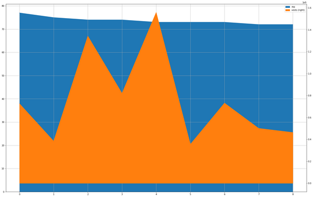
And what we have in front of us is relatively straightforward. Because the merge of the tabular data automatically ranked the results by reputation, we have a nice smooth curve being presented of the relatively small difference in Rep, but you can see that there are some fairly significant differences in the amount of SP represented in this group. The numbers on the right are scaled by 10e9 so while the bottom isn't exactly small, we're talking about nearly 4 times difference between the lowest and the highest.
Since this information is so easy to generate, let's step it up a notch. Let's take an order of magnitude more accounts from each list and see how many accounts can be found on both of them.
RepRT = ResT.drop('reputation', axis=1).sort_values('rep', ascending=False).head(1000)

RepRT.head()
| name | rep | vests | |
|---|---|---|---|
| 513965 | steemsports | 78 | 2.338242e+07 |
| 293626 | knozaki2015 | 77 | 1.012949e+08 |
| 211043 | haejin | 77 | 1.741729e+08 |
| 410136 | papa-pepper | 77 | 2.866042e+07 |
| 193328 | gavvet | 77 | 7.260105e+08 |
VesRT = ResT.drop('reputation', axis=1).sort_values('vests', ascending=False).head(1000)

VesRT.head()
| name | rep | vests | |
|---|---|---|---|
| 512095 | steemit | 35 | 9.003985e+10 |
| 358983 | misterdelegation | 25 | 3.385447e+10 |
| 510769 | steem | 25 | 2.124977e+10 |
| 186110 | freedom | 25 | 1.570402e+10 |
| 70044 | blocktrades | 70 | 9.516259e+09 |
CrsT = pd.merge(RepRT, VesRT)
CrsT.head()
| name | rep | vests | |
|---|---|---|---|
| 0 | steemsports | 78 | 2.338242e+07 |
| 1 | knozaki2015 | 77 | 1.012949e+08 |
| 2 | haejin | 77 | 1.741729e+08 |
| 3 | papa-pepper | 77 | 2.866042e+07 |
| 4 | gavvet | 77 | 7.260105e+08 |
CrsT.tail()
| name | rep | vests | |
|---|---|---|---|
| 279 | greenman | 65 | 6.448829e+07 |
| 280 | ftlian | 65 | 2.335072e+07 |
| 281 | aizensou | 65 | 2.264157e+07 |
| 282 | fulltimegeek | 65 | 7.519966e+08 |
| 283 | storyseeker | 65 | 2.401766e+07 |
The top of the chart doesn't change, but it's good to make sure that we understand what we are seeing.
It's the bottom that's particularly useful here. We know immediately that in the top 1000 most reputed and most vested accounts, 284 are found in both lists. The percentages going up, but we would expect to see that because as you move out of the rarefied reaches of both SP and Reputation, the population increases fairly aggressively.
Keep in mind, whenever we talk about SP or Reputation, we're talking about exponential curves, and they have very aggressive knees.
Let's see what that looks like.
CrsT.plot(kind='area', figsize=(25, 16), secondary_y=['vests'], grid=True)
<matplotlib.axes._subplots.AxesSubplot at 0x2324c763ef0>
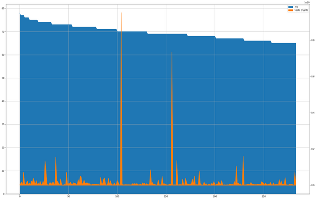
That's a significant spike in the middle. I wonder who that is at a Reputation of about 70?
CrsT.loc[CrsT['vests'] == max(CrsT['vests'])]
| name | rep | vests | |
|---|---|---|---|
| 104 | blocktrades | 70 | 9.516259e+09 |
Oh, it's an exchange.
To be fair, @blocktrades has been a pretty active member of the community with both posts and comments, which is how one manages to get a high reputation – by giving people something to vote on. That works out pretty well.
It is a reminder that we did not filter this list for the accounts that we know are extremely high vest as we often have in the past, but that kind of filtering would not be useful here because part of what we're looking at is whether or not those accounts show up in this context.
Taking the top 1000 Reputation accounts brings us down to Rep 65, which isn't particularly the realm of mere mortals quite yet. You can see that the curve is beginning to flatten out, even among this filtered high vest account representation.
Outside of a couple of really huge outliers, the amount of vesting doesn't seem to have a strong correlation with Reputation at all at this level, either. If anything, it looks very much like some kind of noise function, with just enough occasional spikes to keep interest up. Compare the formations on the left side of the chart with those on the right; things appear to be calling down in terms of dynamic and perhaps there is less overall SP being warehoused, but the spikes are very similar.
Let's do it again, except this time will go up another order of magnitude to 10,000 accounts.
RepRT = ResT.drop('reputation', axis=1).sort_values('rep', ascending=False).head(10000)

RepRT.head()
| name | rep | vests | |
|---|---|---|---|
| 513965 | steemsports | 78 | 2.338242e+07 |
| 293626 | knozaki2015 | 77 | 1.012949e+08 |
| 211043 | haejin | 77 | 1.741729e+08 |
| 410136 | papa-pepper | 77 | 2.866042e+07 |
| 193328 | gavvet | 77 | 7.260105e+08 |
VesRT = ResT.drop('reputation', axis=1).sort_values('vests', ascending=False).head(10000)

VesRT.head()
| name | rep | vests | |
|---|---|---|---|
| 512095 | steemit | 35 | 9.003985e+10 |
| 358983 | misterdelegation | 25 | 3.385447e+10 |
| 510769 | steem | 25 | 2.124977e+10 |
| 186110 | freedom | 25 | 1.570402e+10 |
| 70044 | blocktrades | 70 | 9.516259e+09 |
CrsT = pd.merge(RepRT, VesRT)
CrsT.head()
| name | rep | vests | |
|---|---|---|---|
| 0 | steemsports | 78 | 2.338242e+07 |
| 1 | knozaki2015 | 77 | 1.012949e+08 |
| 2 | haejin | 77 | 1.741729e+08 |
| 3 | papa-pepper | 77 | 2.866042e+07 |
| 4 | gavvet | 77 | 7.260105e+08 |
CrsT.tail()
| name | rep | vests | |
|---|---|---|---|
| 4589 | bliss7 | 54 | 1.780560e+07 |
| 4590 | ozphil | 54 | 4.436549e+06 |
| 4591 | tensaix2j | 54 | 1.034768e+06 |
| 4592 | crypto2day | 54 | 2.609595e+06 |
| 4593 | artific | 54 | 2.166702e+07 |
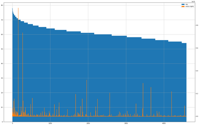
CrsT.plot(kind='area', figsize=(25, 16), secondary_y=['vests'], grid=True)
<matplotlib.axes._subplots.AxesSubplot at 0x2324c76d208>
CrsT.loc[CrsT['vests'] == max(CrsT['vests'])]
| name | rep | vests | |
|---|---|---|---|
| 154 | blocktrades | 70 | 9.516259e+09 |
Looking at the bottom of the list, we are finally down into the range of reputations you could aspire to be among with a concerted effort over several months. 54 is a perfectly reasonable and respectable place in the hierarchy.
The chart is, again, dominated by @blocktrades, to the point I'm starting to think that any kind of analysis going forward that looks at SP is going to have to start filtering out some of these really extreme outliers. At a certain point they just begin masking what might be clearer signal.
Almost 4600 of the 10,000 accounts at the top of both lists are on both lists, which is another indicator that we are down in the realm of the mortals. When we're talking about this kind of range, it's largely everyday people – and functional bots.
Again, look at the vests line as we go from the really sharp knee of reputation descending down into the flats. Beyond a couple of really extreme outliers, and what is a little bit of an obvious bias to holding SP up into the mid-60s of Reputation, things become even more dynamic and spiky. There are vast swaths of relatively low vest accounts punctuated with rather more extreme examples.
One more time into the breach, pumping up things by another order of magnitude and seeing what falls out at the 100,000 account level.
You know already that this will take the graph down into some very basic territory, so let's see what that looks like.
RepRT = ResT.drop('reputation', axis=1).sort_values('rep', ascending=False).head(100000)

RepRT.head()
| name | rep | vests | |
|---|---|---|---|
| 513965 | steemsports | 78 | 2.338242e+07 |
| 293626 | knozaki2015 | 77 | 1.012949e+08 |
| 211043 | haejin | 77 | 1.741729e+08 |
| 410136 | papa-pepper | 77 | 2.866042e+07 |
| 193328 | gavvet | 77 | 7.260105e+08 |
VesRT = ResT.drop('reputation', axis=1).sort_values('vests', ascending=False).head(100000)

VesRT.head()
| name | rep | vests | |
|---|---|---|---|
| 512095 | steemit | 35 | 9.003985e+10 |
| 358983 | misterdelegation | 25 | 3.385447e+10 |
| 510769 | steem | 25 | 2.124977e+10 |
| 186110 | freedom | 25 | 1.570402e+10 |
| 70044 | blocktrades | 70 | 9.516259e+09 |
CrsT = pd.merge(RepRT, VesRT)
CrsT.head()
| name | rep | vests | |
|---|---|---|---|
| 0 | steemsports | 78 | 2.338242e+07 |
| 1 | knozaki2015 | 77 | 1.012949e+08 |
| 2 | haejin | 77 | 1.741729e+08 |
| 3 | papa-pepper | 77 | 2.866042e+07 |
| 4 | gavvet | 77 | 7.260105e+08 |
CrsT.tail()
| name | rep | vests | |
|---|---|---|---|
| 40776 | johnfite | 33 | 82520.899414 |
| 40777 | truthseekker | 33 | 66742.467014 |
| 40778 | kapengbarako | 33 | 25662.241703 |
| 40779 | hbsteemit | 33 | 95787.445843 |
| 40780 | aabraham | 33 | 719718.066746 |
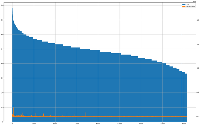
CrsT.plot(kind='area', figsize=(25, 16), secondary_y=['vests'], grid=True)
<matplotlib.axes._subplots.AxesSubplot at 0x2324ebfd0b8>
max(CrsT['vests'])
90039851836.6897
CrsT.loc[CrsT['vests'] == max(CrsT['vests'])]
| name | rep | vests | |
|---|---|---|---|
| 39549 | steemit | 35 | 9.003985e+10 |
And so it begins, the beginning of the end.
And it's the beginning of the end because, besides the fact that we have truly moved beyond the space which is telling us about what high Reputation accounts are involved in, we've moved into the space where the extremely high SP accounts start showing up – and by that I mean one account in particular:
@steemit .
And all the other corporate accounts, because as we saw back at the beginning of this article, they all have raw reputations of zero, and by the calculations which we have been provided, we know that all zero reputations get shifted to 25, because Reputation is designed to originate at Rep 25.
Because the amount of vesting held by @steemit , @misterdelegation , and his kin are so high, there's a ridiculous blip on the charts at 25 Reputation. It pushes everything else down into insignificance, but even so you can see that there is less dynamicism as Reputation continues to fall off past the 25 point.
Until you start getting down to the bottom of the chart, and I'm really not sure what's going on there. Something weird is in the neighborhood. I think you know who we need to call.
Before we do that, let's look at a scatterplot of reputation versus SP. It's not perfect, but it can give you a little bit of a feel for what the distribution looks like from a different angle.
CrsT[CrsT['name'] != 'steemit'].plot(kind='scatter', figsize=(25, 16), x='rep', y='vests', logy=True, grid=True)
<matplotlib.axes._subplots.AxesSubplot at 0x23252a28ba8>
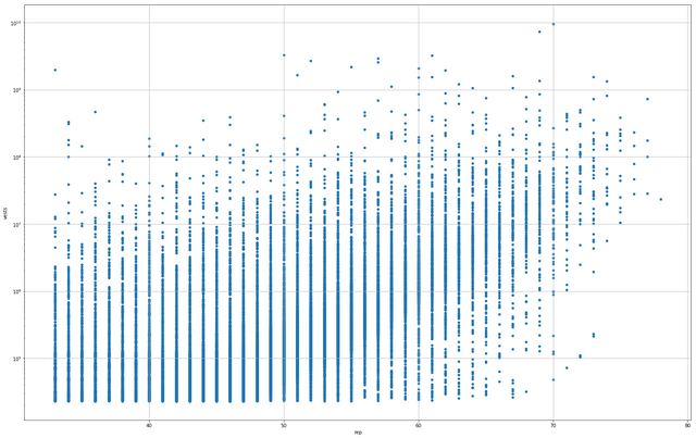
Really, it tells us what we have had pretty heavily reinforced, that the distribution at the bottom is largely exactly that, at the bottom.
Even changing the y-axis to a logarithmic display really doesn't change what we know to be the case. If anything, it reinforces it for the most part in a very heavy-handed way.
This plot does show us that the higher reputation accounts are tending to carry very much the same amount of vests, somewhere between 10e7 and 10e8 while there are a fair scattering of accounts even as low as the early 50s which are actually carrying more SP than those at the top.
I find of the forced vertical lines of the integer transformation to be strangely pleasing. I may be alone in this.
We've looked at the top, now it's time to court the appropriate and look at the bottom.
Bottom-Dwellers
I think we all know what we find at the bottom of a pond, right?
Bottom feeders.
Ecologically, there's no problem with bottom feeders. They serve a useful purpose in the world. They consume the little bits of everything else that the rest of the world misses, and reinject that energy back into the system. When they die.
My original thought was to start with the bottom 1000 of reputations and the top 1000 of SP holding accounts – but my dream was shattered rather quickly, as it became obvious that there were only two accounts on that list.
A chart with two data points on it is very boring. I may be many things, but very boring is not one of the aspirational goals of my life.
Instead, I pumped up the coverage by an order of magnitude, and that has certain side effects. In particular, it means that because of the way that we have sorted the reputation table, the "bottom end" of Rep goes all the way up into the low reaches of 25.
Down in that space there are some very strange account behaviors. Accounts which have been plundered for their SP as vesting transfers, effectively stealing the stake they were created with. Bots which don't interact with people very much in a positive way. Some obvious choices. The usual.
Taken as a whole, however, there are only 40 accounts which exist on both the bottom 10,000 rung of the reputation ladder and the top 10,000 most vested accounts.
I'll be honest, I'm surprised there is that much overlap. I'm not sure what it says that there can be that much overlap.
RepRT = ResT.drop('reputation', axis=1).sort_values('rep').head(10000)

RepRT.head()
| name | rep | vests | |
|---|---|---|---|
| 59937 | berniesanders | -17 | 8.749655e+06 |
| 580751 | wang | -16 | 2.851960e+03 |
| 340682 | matrixdweller | -15 | 4.698676e+04 |
| 92032 | chainflix | -14 | 3.730789e+05 |
| 435071 | r4fken | -12 | 7.235129e+01 |
RepRT.tail()
| name | rep | vests | |
|---|---|---|---|
| 514818 | stellajsteen18 | 25 | 165049.379874 |
| 514830 | stellapowers | 25 | 1026.780133 |
| 514828 | stellanickki | 25 | 1024.052389 |
| 508269 | srokon1234 | 25 | 1024.857985 |
| 514827 | stellamora | 25 | 1032.139056 |
VesRT = ResT.drop('reputation', axis=1).sort_values('vests', ascending=False).head(10000)

VesRT.head()
| name | rep | vests | |
|---|---|---|---|
| 512095 | steemit | 35 | 9.003985e+10 |
| 358983 | misterdelegation | 25 | 3.385447e+10 |
| 510769 | steem | 25 | 2.124977e+10 |
| 186110 | freedom | 25 | 1.570402e+10 |
| 70044 | blocktrades | 70 | 9.516259e+09 |
CrsT = pd.merge(RepRT, VesRT)
CrsT.head()
| name | rep | vests | |
|---|---|---|---|
| 0 | berniesanders | -17 | 8.749655e+06 |
| 1 | davidding | -10 | 4.156951e+08 |
| 2 | elfspice | -7 | 2.359363e+06 |
| 3 | asiahajranajma | -5 | 2.789160e+06 |
| 4 | freeyourmind | -2 | 3.640003e+08 |
CrsT.tail()
| name | rep | vests | |
|---|---|---|---|
| 34 | stefan | 25 | 2.066879e+06 |
| 35 | ssheartofgold | 25 | 1.077192e+06 |
| 36 | ssievert4509 | 25 | 2.948758e+06 |
| 37 | sschechter | 25 | 1.418442e+06 |
| 38 | stephanie | 25 | 2.558245e+06 |
CrsT.plot(kind='line', figsize=(25, 16), secondary_y=['vests'], grid=True)
<matplotlib.axes._subplots.AxesSubplot at 0x23252bc6f28>
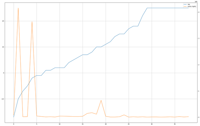
max(CrsT['vests'])
415695090.567864
CrsT.loc[CrsT['vests'] == max(CrsT['vests'])]
| name | rep | vests | |
|---|---|---|---|
| 1 | davidding | -10 | 4.156951e+08 |
And we have a winner! If by "winner" what you mean is "account with the highest SP and one of the lowest Reputations on the entire blockchain. That is – impressive.
@davidding , down there in the mighty -10 Rep zone (which takes some doing, considering that even in the negative space, reputation is scaled by log-base-10), almost a year old – and getting a fat wad of curation SP on a regular basis, if I read the output of steemd right.
This is a very strange part of the world to be looking at.
You can see the plateau of accounts being compressed into the Rep 25 space and you can see that aside from a couple of outliers, there is very little SP kicking around down here. That's pretty much utterly as expected. It's the outliers which are weird.
Epilogue
Have we learned what we set out to learn? That's the question I ask myself every time I post one of these analysis documents; does it communicate something that I didn't know before? Does it give me a better understanding of what's going on around me?
You'll notice in absence of asking the question "is it useful to know this?" I firmly believe that it is useful to know pretty much everything, and if it's not useful, it's interesting and keeps me out of the bars and off the streets at night.
We started by wondering what the overlap is between high SP accounts and high Reputation accounts, and I think we've covered that pretty well. Being highly vested appears to be more correlated with having a high Reputation than vice versa, which doesn't come as a huge surprise.
At the very highest level, the overlap between the highly vested and the highly reputed is pretty sketchy. As you move down and look at larger numbers of accounts, you begin to see that correlation fade, and part driven by some rather extreme outliers, but mostly the noisy gns of the signal of vesting. Once you're down into a space where a goodly chunk of the active accounts on the platform actually live, a couple of extreme outliers dominate the landscape and the rest seems, if anything, either less interested in holding onto or less able to gain SP.
And at the bottom – there is madness, but essential self similarity. A couple of outliers and very little differentiation at the scale we're dealing with.
I expected to see more correlation between higher Reputation and higher SP. Even though there is obviously some, it's much less prevalent than I had hoped to observe. Given the implicit amount of time and effort that a high Reputation demands, purely mechanically, the relative paucity of SP suggests that those with the highest reputations are also fairly well devoted to holding onto a relatively consistent pool and getting rid of the rest, either through power down and selling off or some other mechanism.
Note that I explicitly did not work on calculating delegated versus held SP because that seemed a step more complication than I wanted to get into but this code is certainly capable of taking that into account, using a method which is just like how we calculated the integer Rep of any given account.
Once again we've gone on a deep dive into the actual distribution and functioning of the steem blockchain and I hope that you have found of the company handy even if you haven't found it pleasant.
Drive on, driver!
Tools
- Python 3.6
- Jupyter Lab
- SteemData created by @furion
- MongoDB
- Pandas
And a complete lack of patronage from the Holy See.
Posted on Utopian.io - Rewarding Open Source Contributors
Have my 100%-er Lex, well done!
Thank you for the contribution. It has been approved.
You can contact us on Discord.
[utopian-moderator]
Well, this was.... something.
A lot of that does make sense... many people with high reputations have been upvoted a lot in order to get those high reputations and have continued to stay invested in the system.
Then there are witnesses and the techy guys that earn a lot of stake through other means that doesn't include posting or commenting a lot.
Then there's everyone else... and then the crazy accounts.
It does reinforce the theory that the best way to earn Steem is to have powerful people like you... which really also applies to every other type of currency.
my mind is blown. pixies - where is my mind
love reading your stuff
Hey @lextenebris I am @utopian-io. I have just upvoted you!
Achievements
Community-Driven Witness!
I am the first and only Steem Community-Driven Witness. Participate on Discord. Lets GROW TOGETHER!
Up-vote this comment to grow my power and help Open Source contributions like this one. Want to chat? Join me on Discord https://discord.gg/Pc8HG9x