Deep Learning Note 2 — Part 1 Regularization
In my last post Deep Learning Note1--Neural Networks and Deep Learning I summarized some key points that I found useful from the Coursera course Neural Networks and Deep Learning. In this week I started the second course Improving Deep Neural Networks: Hyperparameter tuning, Regularization and Optimization in the Coursera Deep Learning track. The note in this post focuses on the content of Setting up your machine learning application and Regularizing the network. As a verification, my original post was published on my wordpress blog and I have stated in the original post that it is also published on Steemit. Pictures here are screenshots of the slides from the course.
Fact
Applied ML is a highly iterative process of Ideas -> Code -> Experiment and repeat. We have to accept and deal with it but we certainly should make this process easier. I guess that’s what the machine learning platforms out there are built for.
Before tuning the parameters
One question we have to answer is: what should we tune the parameters on? If you come from a machine learning background, you probably already know that the data should be split into 3 parts.
Train/Dev (Validation)/Test sets
- Tuning the parameters or try different algorithms on the Dev set
- Once you are happy, evaluate on the final test set. The final test set should only be touched once (besides applying the same data transformation you did on the training set).
Split ratio
- Traditionally, we might use 60/20/20.
- In the era of big data, as long as we have enough validation and test records, the percentage doesn’t matter. If your task only needs 10000 records for validation and testing, then the rest can all be used for training. Although, how do you know how many records you need for validation or testing?
Mismatched train/test distribution
One thing to watch out for is that we want our training and testing data may come from the same source/distribution. For example, if we have a cat image recognition application that trained on good-quality cat pics from the web, but most our app users upload low quality/resolution pictures from their cellphone, then we have a mismatch between the training and test data and our model’s performance could suffer because of that. This also seems like a red flag in the requirement gathering and use case analysis.
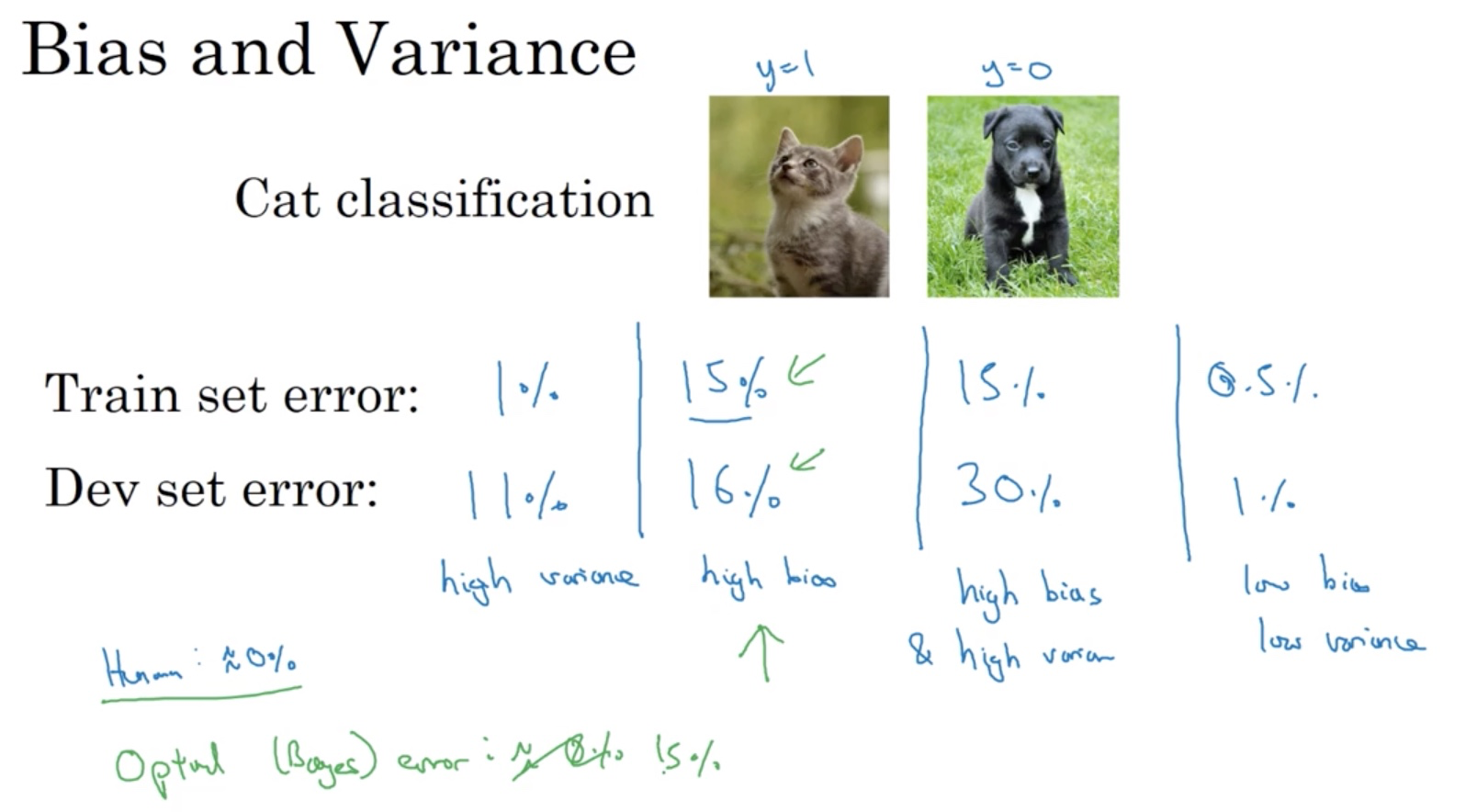
Bias and Variance
One aspect of tuning the model is to handle high bias and/or variance. Unlike the traditional machine learning, they are not necessarily trade-offs in Deep Learning era. Traditionally people talk about bias/variance tradeoff because there were no (or few) good ways to reduce one without increasing the other. However, this is not the case in the deep learning era.
How high is high?
High bias or variance is a relative concept, using the optimal (Bayes) error as a bar. If human gets 1% error, then 15% from the model is too high. But if human gets 13% error, then 15% from machine is not that bad.
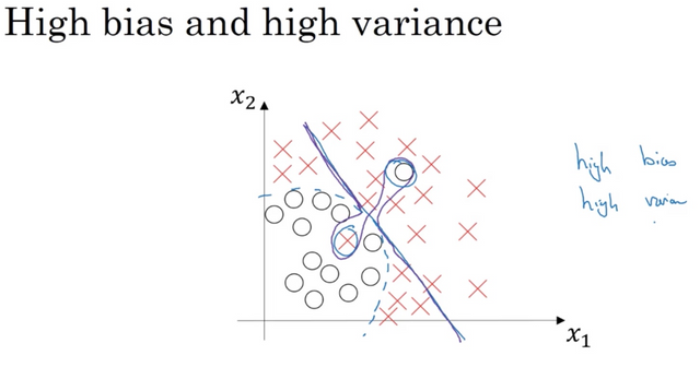
The worst from both world
It is possible that our model could have high bias and variance at the same time, especially in high dimensional space that it can under-fit some regions but overfit some others.
Basic recipe to handle the problem
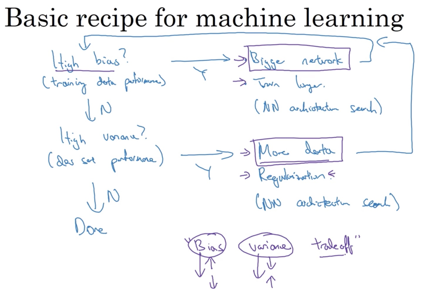
- We start with checking whether the model has high bias on the training data set.
- If yes, we can try bigger network, train longer (or use more advanced optimization algorithms without training longer), or do a search on the NN architecture that suits the problem.
- If no, then we can move on to check if the model has high variance on the dev/validation set.
- Checking high variance is to see if the model is overfitting the training data.
- If yes, then we can try getting more data, applying regularization or doing a NN architecture search that suits the problem.
In the traditional machine learning, people have to carefully handle the situation to lower high bias/variance, risking increasing the other. In NN, as long as we have a well-regularized network, training a bigger network almost never hurts (except for computational time). Getting a bigger network almost always reduces the bias without necessarily hurting the variance as long as we regularize properly. On the other hand, getting more data for the network almost always reduces the variance and doesn’t hurt the bias.
Regularization to reduce high variance
L2 Regularization
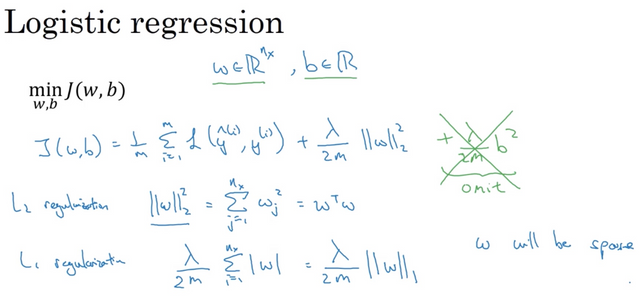
Some people say L1 Regularization compresses the model, but in practice it only helps a bit. L2 are used much more often in practice. The lambda here is called the regularization parameter which controls how much regularization we want to apply. The value of λ is a hyperparameter that you can tune using a dev set. L2 regularization makes your decision boundary smoother. If λ is too large, it is also possible to "oversmooth", resulting in a model with high bias.
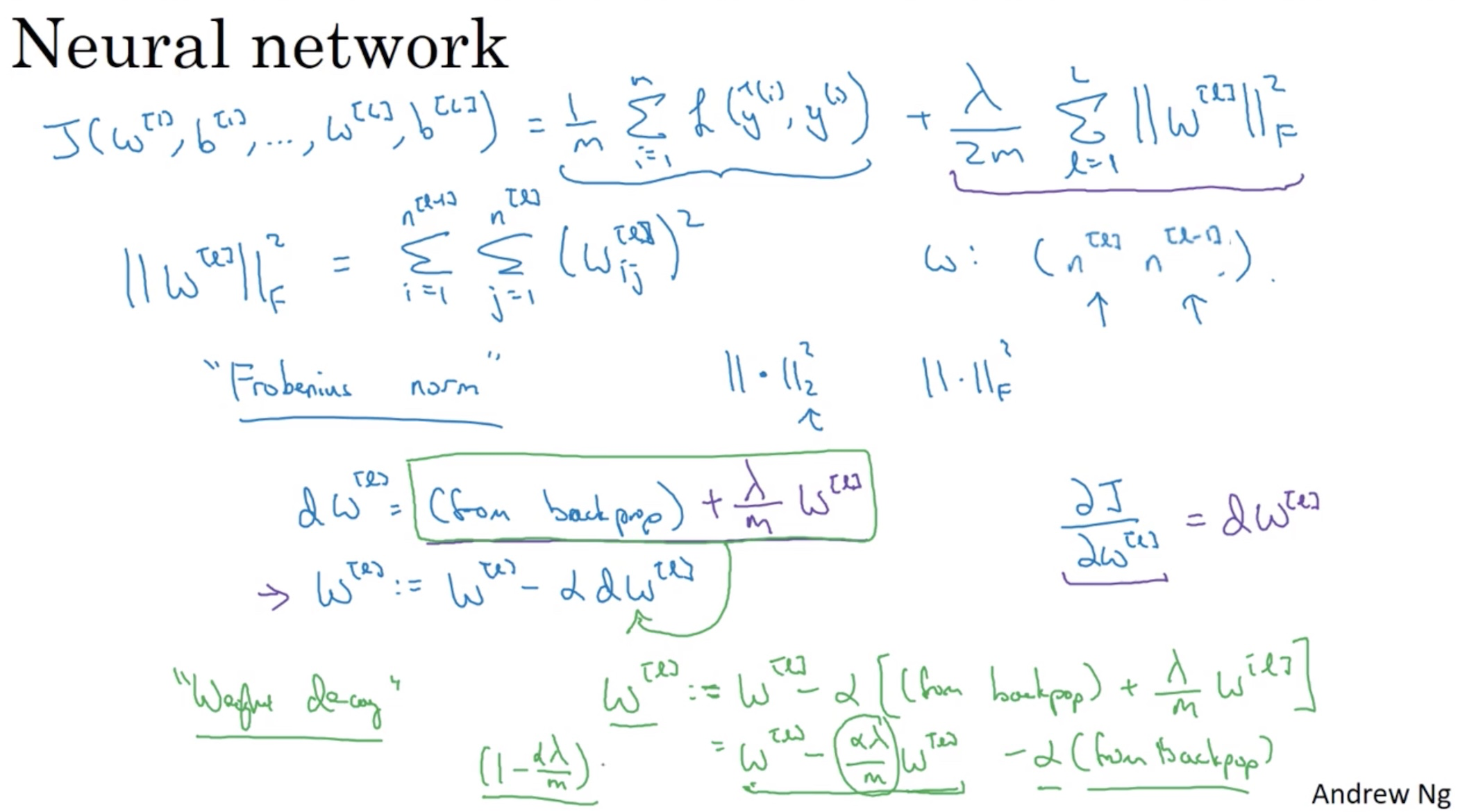
What is L2-regularization actually doing?
L2-regularization relies on the assumption that a model with small weights is simpler than a model with large weights. Thus, by penalizing the square values of the weights in the cost function you drive all the weights to smaller values. With L2 regularization, it becomes too costly for the cost function to have large weights. This leads to a smoother model in which the output changes more slowly as the input changes. L2 regularization is also called weight decay because of the term (1 - alpha * lambda / m) * W shows that the value of W is being pushed to smaller values in each back-propagation (See the screenshot below).
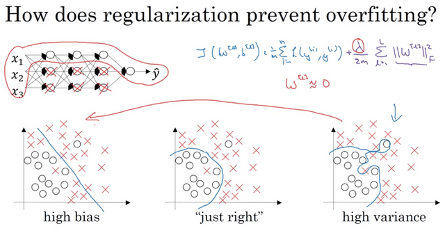
Why does regularization help reducing overfitting?
One (not so accurate but easy to understand) intuition is that if we set a very large lambda, it will drive the W to near 0, much like zeroing out a lot of nodes in the network, resulting in a simpler network. In reality, we still use all the nodes but they just have a smaller effect and we end up with a simpler network.
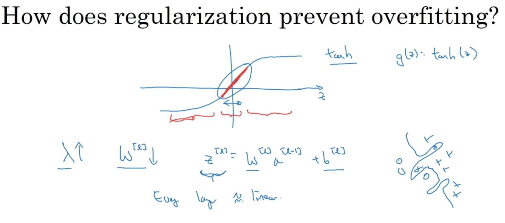
Another intuition is that say we use a tanh function as the activation function, if we increase lambda, W becomes smaller and so does the value of Z. If Z stays in a small range around 0, the tanh is close to linear. If every node or layer is like this, the whole network becomes close to linear, which is simpler.
Dropout Regularization
How does it work?
At each iteration, you shut down (= set to zero) each neuron of a layer with a probability 1−keep_prob or keep it with probability keep_prob. The dropped neurons don't contribute to the training in both the forward and backward propagations of that iteration. Basically when the neurons are shutdown, we treat them as their output are zeros and keep it that way during both the forward and backward propagation.
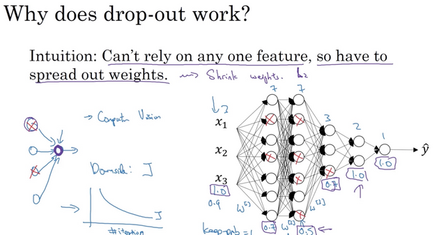
Why does it work?
When you shut some neurons down, you actually modify your model. The idea behind drop-out is that at each iteration, you train a different model that uses only a subset of your neurons. With dropout, your neurons thus become less sensitive to the activation of one other specific neuron, because that neuron might be shut down at any time so it has to spread out the weights. This has a similar affect as the L2 regularization to shrink the weights.
Dropout is used almost by default in Computer Vision because there are just not enough data for computer vision applications. But this doesn’t always apply to other applications. If your model is not overfitting, you shouldn’t apply dropout.
Inverted Dropout
One commonly used dropout technique is called inverted dropout. During training time we divide each dropout layer by keep_prob to keep the same expected value for the activations. For example, if keep_prob is 0.5, then we will on average shut down half the nodes, so the output will be scaled by 0.5 since only the remaining half are contributing to the solution. Dividing by 0.5 is equivalent to multiplying by 2. Hence, the output now has the same expected value. If we don’t scale up, we lose information and the prediction result will be negatively impacted.
In testing phase, we do not apply dropout, otherwise you are just adding noise to your predictions. In theory, we could add dropout to testing but that requires us to repeat the prediction many times and then take an average. It gives similar result but with a higher computational cost.
Other regularizations
Data augmentation
Suppose our model is overfitting and we want to get more data. However, it may not be possible or expensive to do so. One way in Computer vision is that you take your image and randomly transform, rotate or flip it to generate “new” images. It is not as good as getting the real new data (as they are still duplicate in some sense) but it does cost less to get more data.
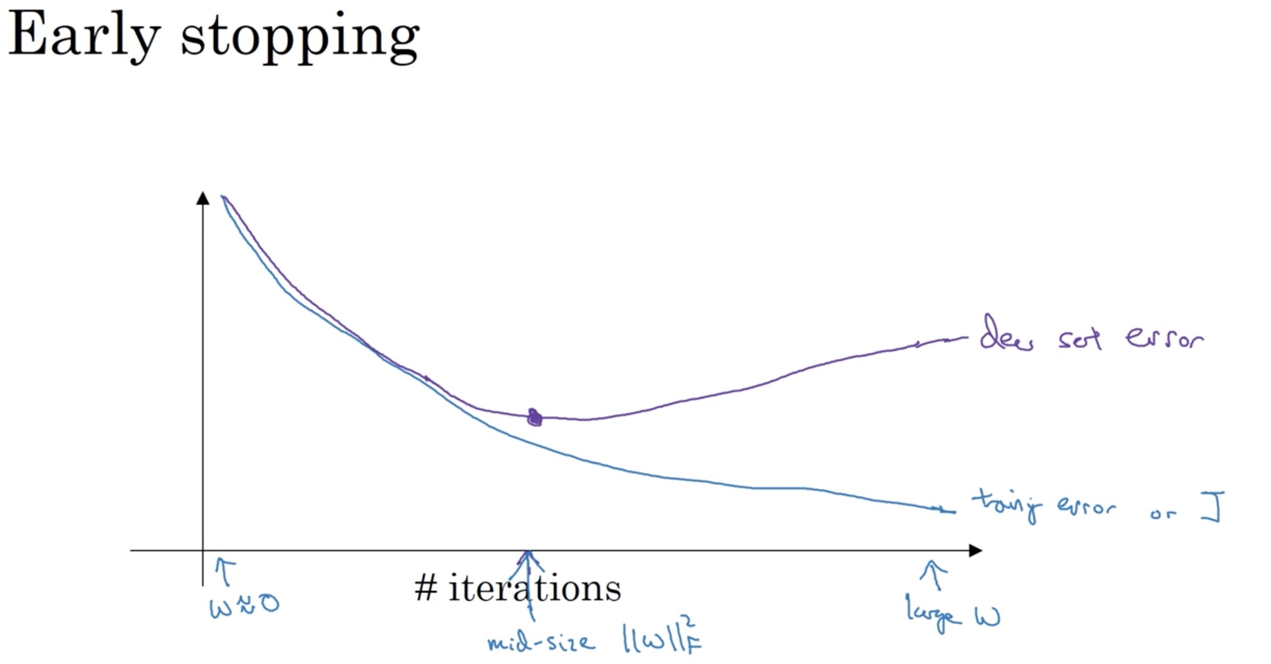
Early Stopping
Stops early in the training process to get a mid-size weight.
But it has a downside as explained below.
Orthogonalization (One task at a time)
In machine learning we already have so many hyper parameters to tune so it’s easier to think about when you have one set of tools to optimizing the cost function J and first focusing on minimizing J. Then as a completely separate task, we want the model to not overfit and we have a separate set of tools to do it.
- Optimize a cost function J
- Using optimization algorithms like gradient descent, momentum, Adam and so on.
- Make sure your model does not overfit.
- Regularization, getting more data and so on.
Using early stopping, it couples the two problems mentioned above and we can no longer work on them independently. An alternative to early stopping is to just use L2 regularization, then we can train the network as long as possible. We do have to try different values of lambda though, assuming you can afford the computation to do so. To be fair, an advantage of early stopping is that you have one less hyper parameter to tune, lambda.
Summary
Note that regularization hurts training set performance! This is because it limits the ability of the network to overfit to the training set. But since it ultimately gives better test accuracy, it is helping your system. Some key points:
- Regularization will help you reduce overfitting.
- Regularization will drive your weights to lower values.
- L2 regularization and Dropout are two very effective regularization techniques.
Reblogged — let’s promote quality content!