Deep Learning Note1--Neural Networks and Deep Learning
Introduction
I recently signed up for the Deep Learning Specialization on Cousera and have just completed the first course Neural Networks and Deep Learning. Although it is recommended for 4 weeks of study, with some backgrounds in Machine Learning and the help of 1.5x play speed, finishing it in 1 week is also achievable. In this post I just want to summarize some of the take-aways for myself and hope it also helps whoever’s reading it. If you are familiar with the implementation of neural network from scratch, you can just skip to the last section for Tips and Best practices mentioned in the course. Note that this is an article I originally posted on my own blog. To prove that this is my own content, I have updated the introduction in my wordpress post showing that I also published it on Steemit. The two posts are now linked together.
Scale of the problem
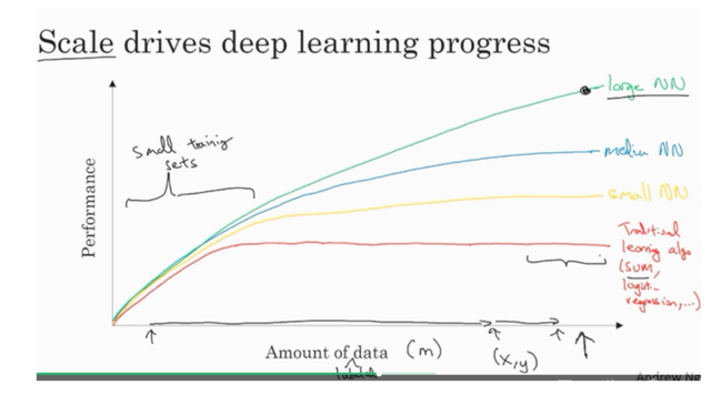
- On small training set, neural network may not have a big advantage. If you can come up with good features, you can still achieve better results using other traditional machine learning algorithms than neural network.
- However, as the amount of data grows, the traditional learning algorithms can hit a plateau while the neural network’s performance keeps increasing. The larger the neural network, the larger the increase.
- As the neural network grows, it takes more resource and times to compute. Many innovation on the neural network algorithms were initially driven by performance requirement.
Question
Why does the traditional algorithm hit a plateau? To be continued...
Logistic Regression as a Neural Network
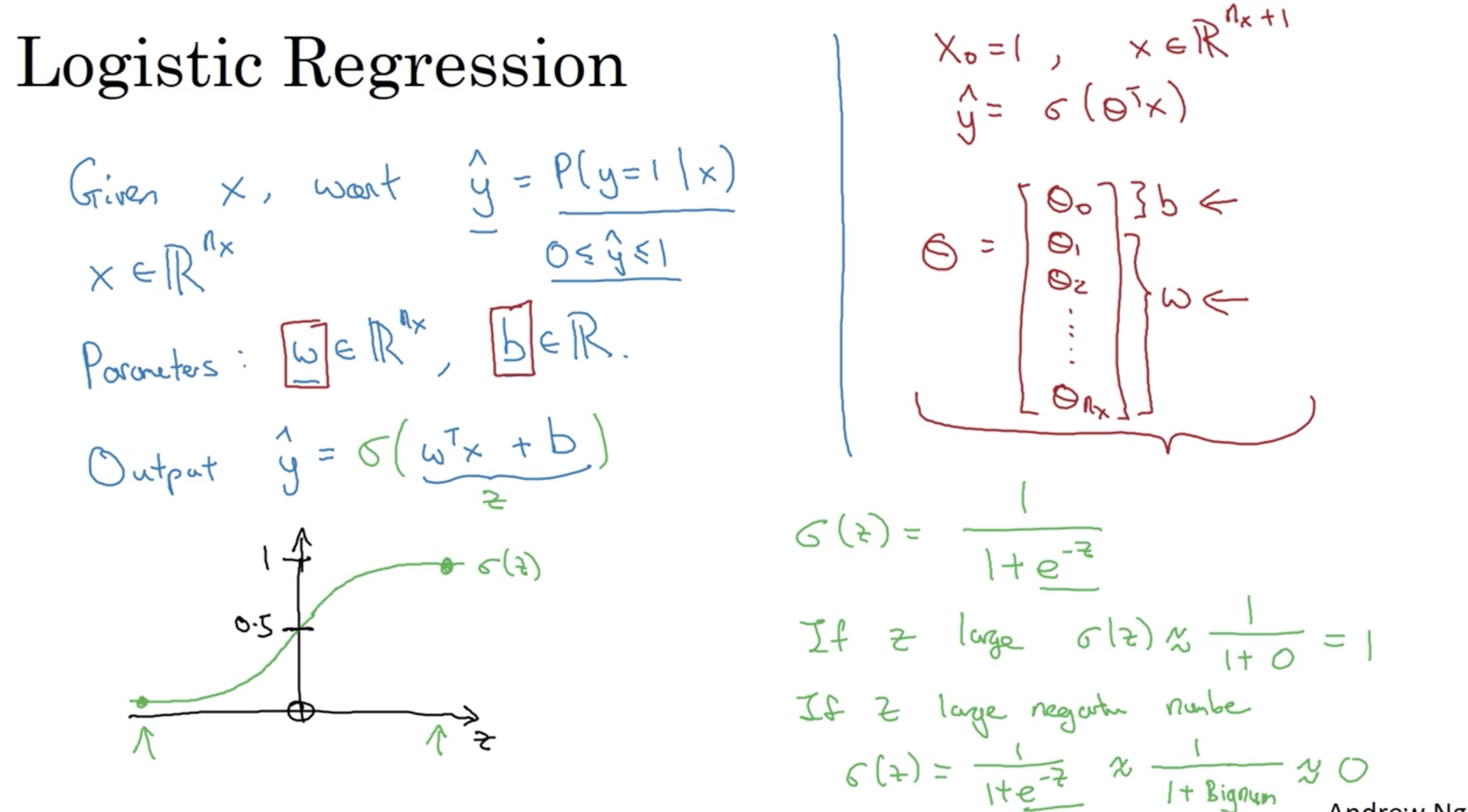
Almost all the books or courses on Deep Learning starts with either logistic regression or linear regression. This is because they can be treated as the simplest neural network with no hidden layer and only 1 neuron.
Using logistic regression as an example, we introduce the following components:
- Scoring function: Z = np.dot(W, x) + b
- Activation function: A = g(Z) where g here is the sigmoid function.
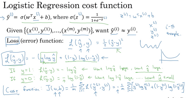
- Loss/Error function: L(y^, y): the function we use to evaluate the difference between y^ and y where y^ is the prediction. Note that loss function is applied on a single example.
- Cost function is the combination of the loss over the whole dataset.
Logistic regression computes the probability of y = 1 given x. There are many choices for the loss function. One of them is the mean squared error but since it is not convex, it could have multiple local minimums so the one used in the course is the cross-entropy loss.
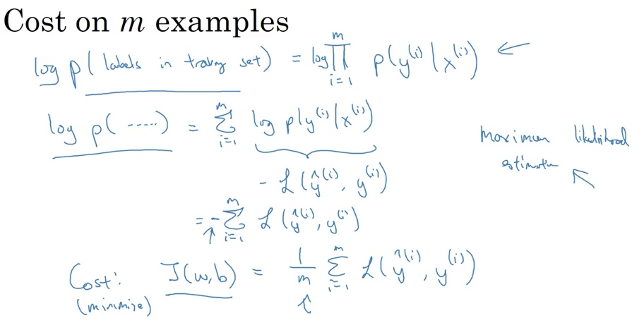
Maximum Likelihood Estimation
If we look at m examples in the training set, assuming that they are independent and identically distributed (iid), training a logistic regression model is computing the probability of the labels given all the x and we are trying to maximize it.
Neural Network
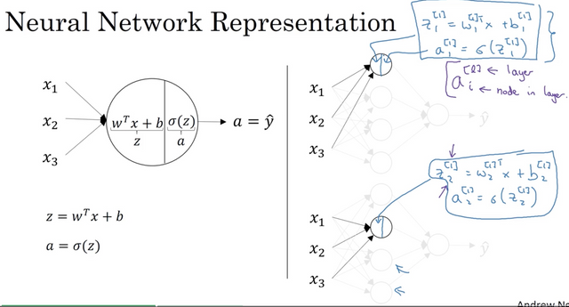
A neural network is really just a collection of connected neurons. Each neuron shares the same compoents:
Zoom out for a more complete view. This is the forward propagation for a single example through the first layer of the neural network.
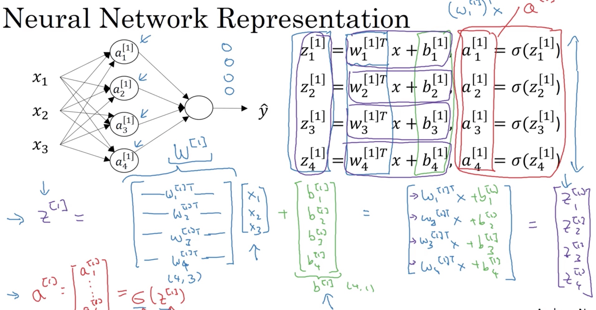
Note that W[1] here represents the W matrix for the 1st layer where each row represents the transpose of w in each neuron. The number inside the bracket [] represent the layer index. The input layer can be treated as layer 0.
Shallow Neural Network
If the neural network has only 1 hidden layer, then we call it a shallow neural network.
Hidden layer
So why is it called hidden? We know the input and output in the training set. However, we do not know those for the layers between the input and output layer so we call them hidden layers.
Deep Neural Network
If the network has more than 1 hidden layer, it’s a deep neural network.
Tips and Best Practices
Notation Cheatsheet
Part 1
This part summarizes the annotations and representations in neural network. I know that there are other forms out there but I really think this is the cleanest way, at least for my brain. The key point is that, anything related with an example is represented in a COLUMN.
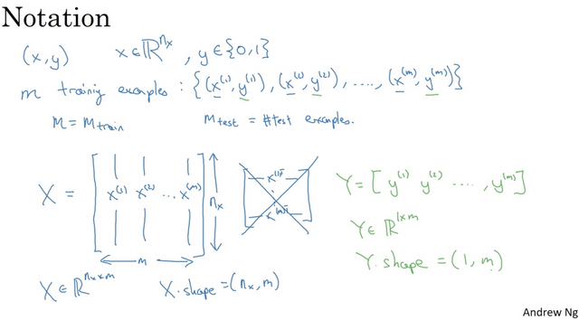
Let’s say that you have m examples and each example has n features. Then the input matrix X is n by m. The target matrix Y is 1 by m. Technically we can think the target Y as a vector, but think it as a matrix of 1 by m will make our life easier down the road.
Another thing to pay attention to is that the index in parenthesis represents something related to the ith example.
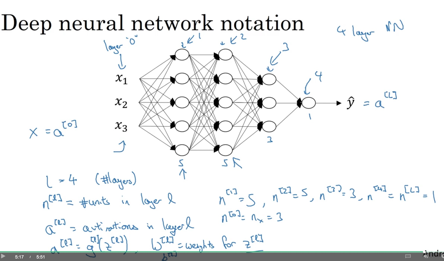
Part 2
One take-away here is the dimension of W and b for layer L. If layer L has n(L) units and layer L-1 has n(L-1) layer, then:
- W is in the shape of n(L) by n(L-1).
- b is in the shape of n(L) by 1.
- dW has the same dimension as W.
- db has the same dimension as b.
Building a neural network
Preprocessing the data (using image classification as an example)
Common steps for pre-processing a new dataset are:
- Figure out the dimensions and shapes of the problem (m_train, m_test, num_px, ...)
- Reshape the datasets such that each example is now a vector of size (num_px * num_px * 3, 1). This is the image_to_vector processing.
- “Standardize” the data. We center and standardize your dataset, meaning that you substract the mean of the whole numpy array from each example, and then divide each example by the standard deviation of the whole numpy array. This will help the gradient descent process.
The whole modelling process (and how to build it from scratch)
The main steps for building a Neural Network are:
- Define the model structure (such as number of input features, number of layers and other hyper parameters)
- Initialize the model's parameters
- Loop:
- Calculate current loss (forward propagation)
- Calculate current gradient (backward propagation)
- Update parameters (gradient descent)
You often build 1-3 separately and integrate them into one function we call model(). We can break down even more to define the activation and propagate function.
How to initialize the parameter
For logistic regression, we can initialize all the parameters (W and b) to all zeros. However, we cannot do this for neural network since it will result in all neuron become identical. If all neuron are identical, we lose the meaning of using a neural work. We have to randomly initialize the parameters to break symmetry of the neurons. As a general rule, we can initialize them in the following way:
- W = np.random.randn((d1, d2)) * 0.01 # we use small value (not necessarily 0.01) here because if we use sigmoid or tanh, the score can be large and the gradient at that place becomes small and slows down the training.
- b = np.zeros((d1, 1)) # b does not have any symmetric issues.
Activation function
The scoring function WX + b is linear but it is the nonlinear output that makes neural networks powerful to learn complex structures in data.
Sigmoid and Tanh function
These two functions both suffer from the problem that when the input value z is very large or small, the gradient of the function becomes close to 0 and thus slows down the training process. Tanh has one advantage over the sigmoid function that the activation value is centred at 0 between (-1, 1), which is easier for gradient descent.
For binary classification, using the sigmoid function as the activation of the unit on the last layer is fine, but for other layers, we may want to consider the following two types below.
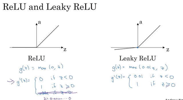
Rectified Linear Unit (ReLu)
This is one of the most widely used activation function in practice. A = max(0, Z)
Leaky ReLu
Performance and Code Quality
- Use vectorization whenever you can. It will speed up the computation drastically.
- DO NOT use numpy 1-D array. It may cause unexpected bug down the road. Even if the data is a single row or column, use a matrix to represent it (either 1-by-N or N-by-1).
Hyper-paratemter tuning
Learning rate
A good learning rate can help the network avoid getting stuck in a local minimum. One mechanism is called Bold Driver as described below:
To resolve this you can check the value of the error function by using the estimated parameters of the model at the end of each iteration. If your error rate was reduced since the last iteration, you can try increasing the learning rate by 5%. If your error rate was actually increased (meaning that you skipped the optimal point) you should reset the values of Wj to the values of the previous iteration and decrease the learning rate by 50%. This technique is called Bold Driver.
Aside from this, when we are setting the initial learning rate, we want to try out a range of parameters. We may want to include a collection of them with different magnitude like (0.1, 0.01, 0.001 and so on).
The number of units in the hidden layer
There is no hard rules about this but some general guidance from this Quora post:
- The number of hidden nodes in each layer should be somewhere between the size of the input and output layer, potentially the mean.
- The number of hidden nodes shouldn't need to exceed twice the number of input nodes, as you are probably grossly overfitting at this point.
Debugging the network
If we see that the network is not converging, even after changing the learning rate and other parameters, then we need to dig into the data representation to make sure they have the signal we expect. Before we get all fancy with regularizations or other tools, we want to go back to the data first. Data is where all the gold is. The neural network is just digging the gold. If it’s not working, it is probably because of where we are digging.
Noise and Signal
Neural network is just weights and functions. We want the weighted sum to highlight the signal, not the noise. The way we process our data could result in both ways. Look at your data representation and think about if the current way magnified the noise too much. The more we can increase the ratio of signal/noise, the more we can help NN to cut through the obvious stuff and focus on the difficult part. This is what framing the problem is all about.
Production system
Trade the prediction for performance. If we have more data and the algorithm is made faster, we can cover more ground and achieve more.
Overall
The technique of framing the problem is very general. When we have a new dataset, we are going to need to come up with a new predictive theory and then tune our model and dataset to make the correlation in your dataset most obvious to the network so it can both predict quickly and accurately. Each time we do this, we will see performance increase on the network.
This actually shows that even with NN, we still need to do some feature engineering.
Thanks for reading :)
Congratulations @steelwings! You have completed some achievement on Steemit and have been rewarded with new badge(s) :
Click on any badge to view your own Board of Honor on SteemitBoard.
For more information about SteemitBoard, click here
If you no longer want to receive notifications, reply to this comment with the word
STOPCongratulations @steelwings! You have completed some achievement on Steemit and have been rewarded with new badge(s) :
Click on any badge to view your own Board of Honor on SteemitBoard.
For more information about SteemitBoard, click here
If you no longer want to receive notifications, reply to this comment with the word
STOPHowever, we would like to see some visual confirmation that this and the website you took it from are both in fact you. There is a LOT of spam and theft on this site, so we need to be sure. You can do this by simply updating your introduction post =D
Thanks @mobbs. I have updated my introduction on both sides. They are now linked together. https://jznest.wordpress.com/2017/08/19/deep-learning-note-neural-networks-and-deep-learning/
Awesome! Welcome to the community, hopefully see you in the chat some time =D
@steelwings Excellent Tale. Awesome you ended up in the position to hustle your way out of your respective condition.