Hello all my steemit community friends. I want to express my warm greetings to all of you. It's me @leoumesh and today I am gonna be giving a very brief introduction on Skewness in statistics.

So lets begin with the very topic.

Designed from Adobe Photoshop CS6

Before learning about skewness, lets get some intro on central tendency.

Central Tendency

One of the foremost objective of statistics is to get one single value that represents the property or characteristics of the entire data. We call such a value as central value. This value represents a group of value and this value lies somewhere in between the two extremes i.e. the largest and the smallest items. For this reason, it is also known as central value. The process for obtaining a central value from the entire data is known as central tendency. The most popularly used measures for central tendency are:

1. Mean

The most popular widely used measure of representing the entire data by one value is the mean. Its value is obtained by adding together all the items and by dividing this by the total number of items. It is the simpliest average to understand and the most easy one to compute which is based on each and every observation. It is represented by and is calculated by:

=
where,

= Sum of all items

N= Total number of items

2. Median

The middle of a set of numbers is the median. It divides an ordered set into two equal parts half. 50% of the number will have value less than the median and 50% will have value greater than the median. Thus, if data are arranged according to their magnitude in ascending or descending order, the median value is half way through it.

For example, if we have 7 students with marks 28, 31 , 27 , 45 , 43 , 52 , 38, median of the mark obtained by those students can be found by ranking the marks and taking the 4^th figure in the order of magnitude. The mark thus ordered will be 27 , 28 , 31 , 38 , 43 , 45 , 52 and the median will be 38.

Median is especially useful in case of open end classes and is the most appropriate average in dealing with qualitative data. Median can also be obtained graphically and is rigidly defined. The methods for finding median are:

i. Finding median of individual data

The data is first arranged in the ascending or descending order of magnitude. The total number of item (N) is counted. The median is then calculated using the formula:

Position of median = items

Thus position of items give the value of median.

ii. Finding median of discrete data

The data is first arranged in the ascending or descending order of magnitude. The total number of item (N) is counted. The median is then calculated using the formula:

Position of median = items

Now, we look in the cumulative frequency column and find that total which is equal to or greater than position of median and determine the value of the variables corresponding to it. This value gives the median.

iii. Finding median of continuous data

Here in continuous series, the data is given in terms of class or range of values. To find median, the data is first arranged in ascending or descending order of their magnitude. The total number of items (N) is calculated by constructing table containing cumulative frequence. Then we apply the following formula :

Position of median = N / 2

Then we look all the cumulative frequency column and find that total value which is either equal to (N/2) or next higher to that and determine the class of the variable for exact value of median and using the following formula :

Median =
where,

L = Lower limit of median class
cf = Cumulative frequency of the class preceding the median class
f = Simple frequency of the median class
h = The range of median class

3. Mode

The mode or modal value is that value in a series of observations which occurs maximum number of times. The mode of distribution is the value at the point around which the items tend to be most heavily concentrated. In other words, the value having maximum frequency in the data is called mode. Moreover, mode is the easiest one to compute and understand. It can be found even in open end classes and can be determined graphically also.

i. For finding mode of individual & discrete series

The value occuring maximum number of times is the modal value.

For example, in the series of marks obtained by student which is

10, 27 , 24 , 12 , 27 , 20 , 18 , 15 , 30 , 27

Here 27 occurs maximum number of times i.e. 3, hence the mode = 27.

ii. For Bi-modal data

If there is two mode or more than two mode in the series of data , model is ill-defined. Then its value is calculated by an Empirical relation:

Mode = 3 * Median - 2* Mean

iii. For finding mode of continuous series

First of all, the modal class is determined by inspecting which class has the maximum number of frequency. Then the following formula is used to get the mode value :

Mode =

where,

L = Lower limit of the modal class
f₁ = Frequency of modal class
f₀ = Preceding frequency of modal class
f₂ = Succeeding frequency of modal class
h = The class interval

Note :- In the process of finding mean , median and mode for continuous series, class should be of equal range and exclusive.

If you want to learn a bit more about central tendency, you can read my friend @bikkichhantyal article on Normal distribution. Please click here.

---

Standard Deviation

The standard deviation is the most important and widely used measure of dispersion or variability. Dispersion means scatter or spread or variation. Dispersion provides the idea of homogeneity or heterogeneity of the distribution. It is different than central tendency because central tendency is itself inadequate to describe the distribution. The standard deviation is represented by SD or . The formula for standard deviation is :

1. For individual observations

=
where,
n = Total number of items
= Mean

2. For discrete or continuous observations

=
where,
N = Total number of items
= Mean
f= frequency

---

Skewness

The measure of central tendency tells us about the concentrqation of the items about the middle of the distribution and the measure of dispersion gives us an idea about the scatterness of the items about the measure of central tendency. But the distribution may differ in nature and composition though they have same central tendency and dispersion.

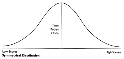
Skewness means "lack of symmetry". The main purpose of studying skewness is to have an idea about the shape of curve which we can draw with the help of the given data. It measures the degree of departure from symmetry. It is used to determine the nature and extent of the concentration of the observations towards higher or lower values of the variables. If in a distribution mean = median = mode , then that distribution is known as symmetrical distribution and it is called a skewed distribution. Such a distribution could either be positively skewed or negatively skewed.

Image Source :floridaschoolleaders

It can be found from the above diagram that in a symmetrical distribution the values of mean, median and mode coincide. The spread of the frequencies is the same on both sides of the center point of the curve.

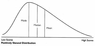
1. Positively Skewed Distribution

Image Source :floridaschoolleaders

In a positively skewed distribution, the value of the mean is maximum and that of the mode is least, the median lies in between two. In the positively skewed distribution, the frequencies are spread out over a greater range of values on the right hand side than they are on left hand side.

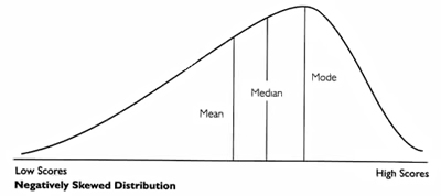
2. Negatively Skewed Distribution

Image Source :floridaschoolleaders

In a negatively skewed distribution, the value of the mode is maximum and that of the mean is least. The median lies in between the two. In the negatively skewed distribution, the frequencies are spread out over a greater range of values on the left hand side than they are on the right hand side.

Properties of skewness

The distribution is skewed if,

1. The value of mean, median and mode do not coincide i.e.

2. First Quartile and Third Quartile are not equidistance from median i.e

3. The sum of deviations from median is not equal to zero.

4. Frequencies are not equal in either side of the mode.

5. The curve of frequency distribution is not symmetrical (bell-shaped).

Measure of Skewness

One of the popular measure for finding skewness is Karl-Pearson coefficient of skewness. IT is the measure of skewness based on mean, median and mode. It can be used for qualitative data and data having open end classes.
Karl-Pearson coefficient of skewness is the difference of mean and mode divided by standard deviation. It is denoted by S_KP and is given by:

SKP = ..........(i)

If mode is ill-defined then,

Mode = 3 * Median - 2* Mean
Hence,

..........(ii)

The Karl Pearson's coefficient of skewness computed from (i) lies between -1 nad +1 but computed from (ii) lies between -3 and +3.

Interpretation of Karl Pearson's coefficient of Skewness

i. If = 0 , the distribution is symmetrical (Not skewed)

ii. If > 0 , the distribution is positively skewed (Right skewed)

iii. If < 0 , the distribution is negatively skewed (Left skewed)

Now we will do example of skewness using Karl Pearson's method.

Let consider the age of children living in a particular society are 2 , 3 , 6 , 9 , 15. Now we have to find the Karl Pearson's coefficient of skewness from these data. So lets begin ahead.

X	X2
2	4
3	9
6	36
9	81
15	225
= 35	= 355

Now,

= 35 , , n=5

= = 35 / 5 = 7

= = = 5.656

Here, mode is ill defined because all numbers are unique and all have frequency 1.

Median = = = 3^rd item = 6

= = 0.53

Here S_KP = 0.53 > 0. Hence the distribution is positively skewed.

Kurtosis

It is the measure of peakedness or flatness of curve of the given distribution. It gives the shape and nature of the middle part of a symmetrical distribution as compared to normal distribution. Kurtosis is characterized with reference of moderate type of curve (normal).

Types of Kurtosis

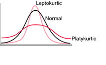
The three types of kurtosis are as follows :-

Image Source : datascienceconcepts

i. Letokurtic Curve

Frequency curve of a distribution is more peaked as compared to mesokurtic (normal) curve is called leptokurtic curve. It has a very peaked top.

ii. Mesokurtic Curve

Frequency curve of a distribution is neither peaked nor flat is called mesokurtic curve. It is also called normal curve i.e. no kurtosis. Kurtosis is determined with reference to this curve.

iii. Platykurtic Curve

Frequency curve of a distribution is more flat as compared to mesokurtic (normal) curve is called platykurtic curve. It has a very flat top.

---

Thanks for reading this article. Please feel free to cooment below.

---

References

1. https://statistics.laerd.com/statistical-guides/measures-central-tendency-mean-mode-median.php

1. https://floridaschoolleaders.org/general/content/nefec/dafil/lesson2-5.htm

2. Mathematical expression coded on : http://www.quicklatex.com/

---

steemstem

steemstem is a community driven project which seeks to promote well-written and informative Science, Technology, Engineering and Mathematics ( STEM ) posts on Steemit. The project involves curating STEM-related posts through upvoting, resteeming, offering constructive feedback, supporting scientific contests, and other related activities.

DISCORD: https://discord.gg/j29kgjS