Normal Distribution: A Simple Introduction
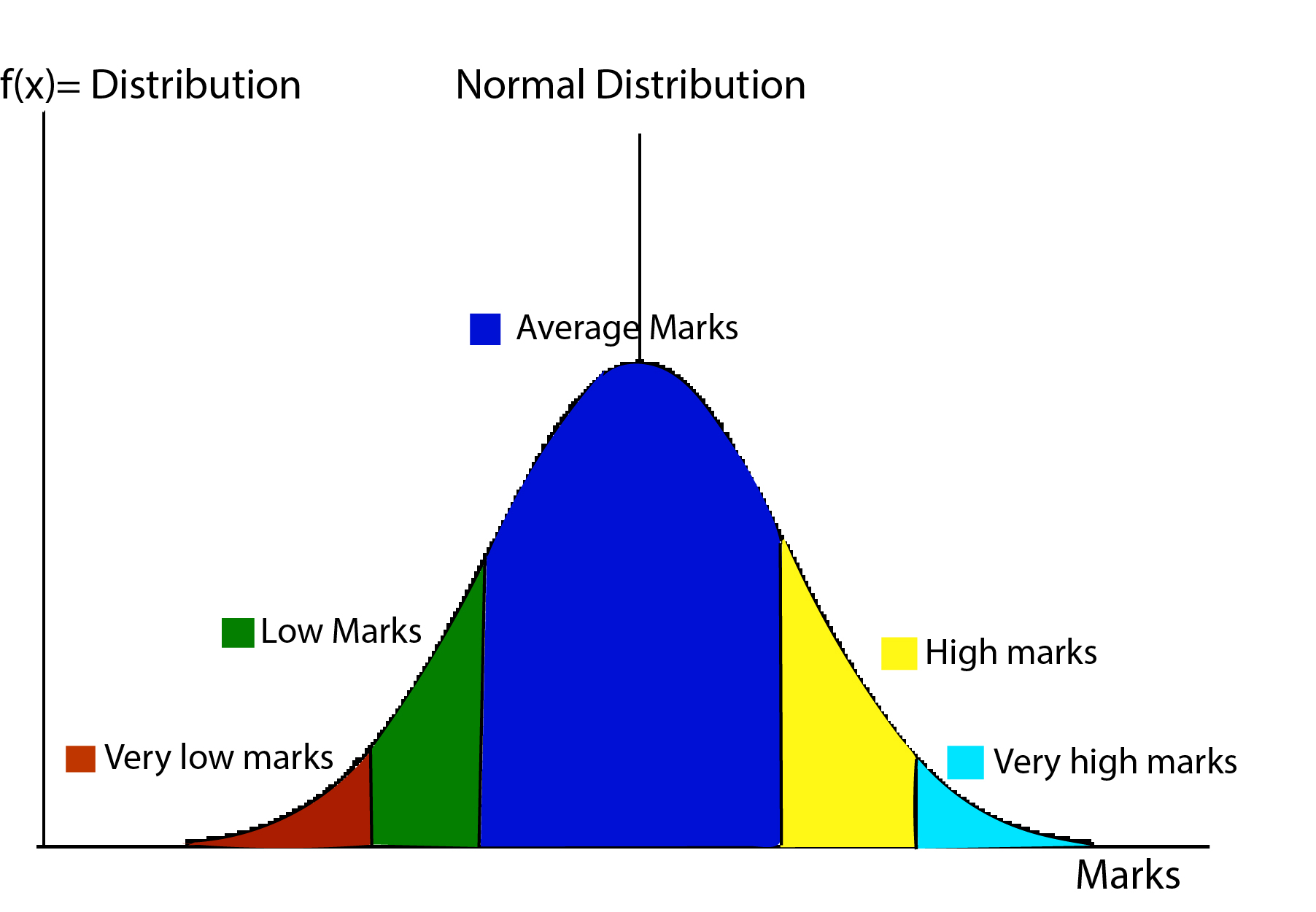
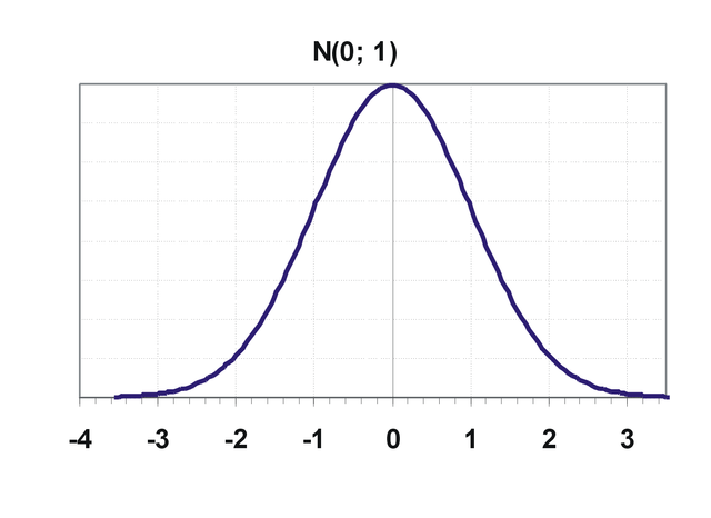
Hey Steemians, you may have realized that there are very few students getting very high and very low marks in your class. The most of the students score around average in the exam The distribution of score obtained in the exam can be modeled approximately by the Normal distribution. The normal distribution looks like following.
The marks are in discrete i.e. whole number, but if it large in number then it can be approximated by continuous curve like above.
Along with marks, the height of people in Steemstem community, the weight of people in your college, IQ scores, the life of turbine blades, error in measurement and so on are beautifully approximated by the normal distribution. It is so consistent with the nature that:
Mathematicians take it as an empirical fact and experimentalists take it as a mathematical fact.
- Henri Poincare(you may have heard about Poincare conjecture)
It was first discovered by De Moivre in 1733 AD. It is also called Gaussian distribution as Gauss used this distribution for characterizing measurement errors. It is a bell-shaped curve so it is often called bell curve.
Preliminary Section:
You need to know certain things for the better understanding of the post. If you have already taken basic statistics course or studied on your own, You may skip this section.
Mean:
Here,
x= Individual elements of data set.
N = Total number of observations.
For example:
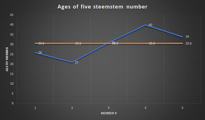
I asked the age of five random members of Steemstem community. The data set I got was:
26,21,31, 40,34
= 30.6 year
It is a single value for the representation of center of data.
To give you graphical perspective, plot the values of ages in the y-axis. Then, the mean line is the horizontal line from which the sum of the square of the distance between points of data sets and the mean is minimum.
To give you physical perspective, let the car travel on a road with velocities v1,v2,v3,v4,v5 for an equal interval of time t. Then, the uniform velocity with which the car should travel to cover the same distance in same time is the mean of the velocities.
There are also other measures of central values like harmonic mean, geometric mean, median, mode, etc.
Standard deviation:
The above subsection is basically about the central location. Standard deviation gives second characteristics of data discussed earlier, i.e. dispersion. How are the data dispersed or deviated from the central location? One former idea may be to add all the deviation from the mean and divide that by the number of observations. If we do that, we will get zero. But, we should consider deviations in both above and below mean. In standard deviation, deviation of each data from mean is squared and averaged. For the same unit as in the observation, the square root of this value is taken.
It is simply root mean square deviation from the mean.
and for individual series,
The data set below is the percentage I got in 6 semesters exams.
80,85,81,77,83,75
= 3.38
Now, we got the value of standard deviation. What can we say about the dispersion of the data? Actually, nothing. The standard deviation gives the deviation. But, it is important to compare it with mean. Now, with the comparison with mean, we can find the coefficient of variation. The coefficient of variation of two data set can be compared to know which data is more dispersed.
Probability:
Probability is the measure of the likelihood of the event. Consider in your college, there are 30 students. Out of them, 20 are females. If you randomly select one person, what is the probability that the person is female?
Random variable:
Consider a random process, flipping of the two coins at a time. The possible outcomes are {H,H}, {H,T},{T,H} and {T,T}. These outcomes can be mapped into numbers. Then these can be denoted by the random variable.
Let, random variable X be the number of tails we get from tossing two coins. Then,
{H, H} is mapped to 0
{H,T}/{T,H} is mapped to 1
{T, T} is mapped to 2.
In above example, the random variable X can only take values like 0,1,2, ... values. So, it is discrete random variable.
Examples:
If we measure the height of people, random variable X(x) = x, x is any positive real number.
Observe the birth of 500 babies in the hospital. The number of baby girls can be a random variable, where it can take discrete value from 0 to 500.
Probability Distribution
In the coin toss example above, the random variable i.e. number of tails can have different values. For each value, there is a probability of occurrence. If we plot, tabulate or graph the possible values of the random variable to the probability of occurrence, it is called probability distribution.
For simplicity, let's tabulate the probability;
| Possible outcomes | Probability |
|---|---|
| P(X=0) | 1/4 |
| P(X=1) | 2/4 |
| P(X=2) | 1/4 |
If we add all the possible outcomes of a random variable, we get sum 1.
Main Section:
What is normal distribution?
If we simply plot the value of x in x-axis and f(x) in the y-axis, we can get the bell curve.
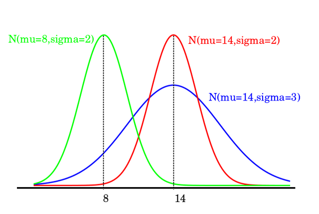
The red and green curve has the same standard deviation, so the width is same. But, they have different means, so centers are different.
The blue and red has same mean but different standard deviation, so their center is same but the width is different.
The function above may look strange at first. But, it is not so common but fairly used function in physics and mathematics. Even its given a special name called Gaussian function. The term apart from exponential is simply normalizing factor i.e. coefficient to make integration unity. This can be proved in few steps using gamma function.
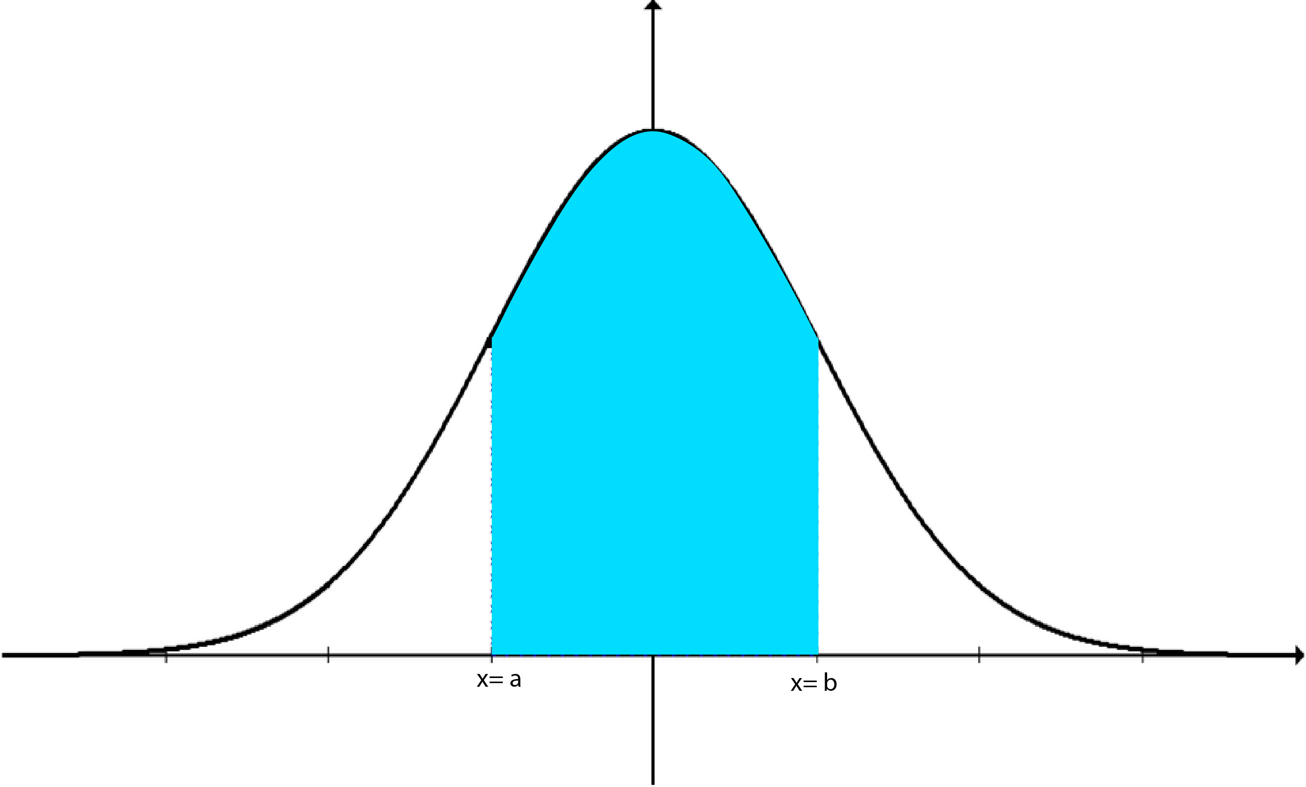
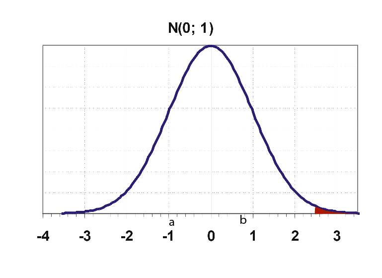
The area enclosed by the curve and two vertical lines x=a and x=b gives the probability of finding the values in between a and b.
Why normal distribution?
As discussed earlier, normal distribution approximates many real-world cases so well. This is normal distribution doesn't mean other distributions are abnormal. Other distribution like binomial distribution, Poisson distribution etc. do really well approximation in their realm. But, even these distribution can be approximated by the normal distribution. For large values of n, it's tedious to calculate values using the binomial distribution. In such case, the normal distribution may be employed to solve the problem easily. All the sampling distributions like t-distribution, chi-square distribution etc. converge towards normal distribution for the large values of n. By historical point of view also, this is most important distribution. Many research inferences are based on modeling using the normal distribution. In mechanical engineering(which is my study field), the control limits are set for quality control using the normal distribution. The measurement error which is integral in case of experimental physics follows the normal distribution.
Standard normal distribution?
We now know that the shape of normal distribution depends upon mean and standard deviation. Different data from observation have different means and standard deviation, so they have different shapes. In principle, we can calculate the probability for each case using integral above but its really tedious work. Moreover, the above integral(containing pdf) cannot be integrated directly. It needs to solved using numerical integration. So, it is logical to make a standard normal distribution and have values of the area for different values of the normal random variable.
We take the special case of the normal distribution with mean zero and the standard deviation unity as standard normal distribution. Every normal distribution can be converted into standard form. In doing so, we should convert the random variable X into something called z-score.
Where z is given by;
Characteristics of standard normal distribution
Z ~ N(0,1), standard normal variable follows the normal distribution with mean zero and standard deviation unity.
The curve is symmetric about line z =0.
Area rule:
Area property of standard normal distribution is most important property.
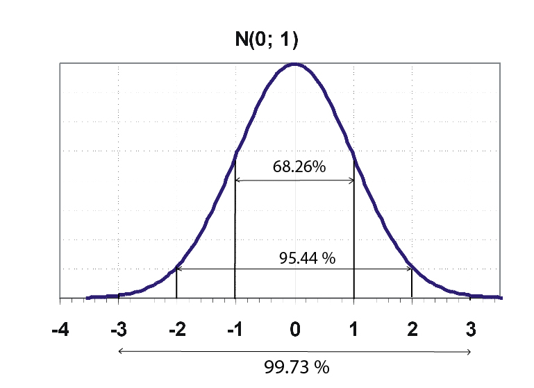
a. The area under the standard normal curve in between ordinates z =-1 to z =1 is 0.686. That means this area covers 68.26% of the observations.
b. The range Z = -2 to 2 covers 95.44 % of the observations.
c. The range Z = -3 to 3 covers 99.73 % of the observations.
The value of Z can extend from negative infinity to positive infinity but for the practical purpose, we often use the area covered by -3 to 3 range as 100%.
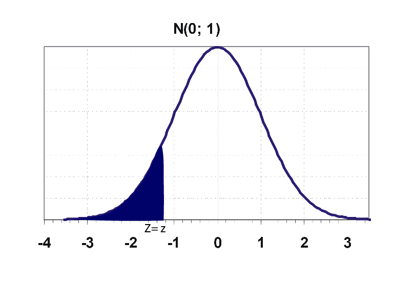
- We have the values of the area for every z as;
- If we have to find the area in between let's say from z=a and z=b(b>a) then,
F(a) gives the area from negative infinity to z=a.
F(b) gives the area from negative infinity to z =b.
F(b) - F(a) gives the area from z=a to z = b.
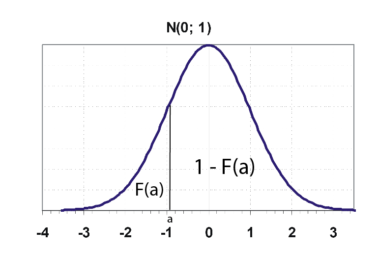
- Conventionally, F(a) gives the area left of z=a. To find the area of right to z=a;
F(-a) = 1 - F(a)
- Mean = Median = Mode = 0
Example
In a School Leaving Certificate level examination in Nepal(grade 10), the mean percentage scored by students is 50 % and the standard deviation of percentage obtained is 12%. If 5 lakhs of students appeared in the examination, calculate the number of students who got the distinction (at least 80%) is the examination. Assume that the distribution is normal.
Solution:
Calculating z score;
for distinction;
= 1- P(z < 2.5)
= 1 - 0.9938
= 0.0062
No. of students securing distinction = 0.0062* 500000 = 3100 students.
In this article, I limited the content up to basics of the normal distribution. Previously, I had the mindset to cover the real applications of normal distribution too. But, this post is already very long. So, in next article, probably I will write about inference using normal distribution, use of normal distribution in my field i.e. mechanical engineering, and other applications.
References
Yamane, T. (1973). Statistics: An introductory analysis.
Brownlee, K. A. (1965). Statistical theory and methodology in science and engineering (Vol. 150, pp. 120-131). New York: Wiley.
Budhathoki, T.B. (2011). Probability and Statistics for Engineers. Kathmandu: Heritage Publications.
Altman, D. G., & Bland, J. M. (1995). Statistics notes: the normal distribution. Bmj, 310(6975), 298.
https://www.mathsisfun.com/data/standard-normal-distribution.html
http://www.statisticshowto.com/probability-and-statistics/normal-distributions/
Reference mathematical tools
Microsoft Excel
www.quicklatex.com
steemstem:
SteemSTEM is a community driven project which seeks to promote well-written and informative Science, Technology, Engineering and Mathematics posts on Steemit. The project involves curating STEM-related posts through upvoting, resteeming, offering constructive feedback, supporting scientific contests, and other related activities.
DISCORD: https://discord.gg/j29kgjS
follow me @:












Being A SteemStem Member
Your post gave an incredible post-traumatic stress to my statistics classes last year :P but you explained it all very well!
I'm a vet student so i don't usually use statistics unless i go into epidemiology, i actually just learned how to work with a program called Epiinfo which correlates data between many epidemiology studies, it shows p-value we use the null hypothesis, etc.... you know what I'm talking about
Are you also going to explain Poisson and binomial distributions? ( i think this is what they are called)
Thank you for your encouraging comment. That is simply hypothesis testing. Normal distribution is for continuous random variable and Poisson and Binomial distribution are for a discrete random variable. They are relatively easy to explain. I think I will explain those.
In future, Maybe, I will also request volunteers from steemstem members in data collection and analyze data to find out various inferences. That would be interesting I guess.
You forgot to add to add sup and sub-scripts to your sigma. But the rest is fine :)
Thank you !!