Which Team is Better and Why? Part I: Using geospatial adjustment computations to rate ice hockey teams.

Which Team is Better and Why? Part I: Using geospatial adjustment computations to rate ice hockey teams.

Mack G. Stevens
Rader School of Business
Milwaukee School of Engineering

April 2017

Abstract
Although least squares mathematical solution techniques have been employed to rate sports teams since the late 1970's, they have been primarily used to create ranking profiles that are non-qualified with respect to their embedded precision properties. This paper presents a short primer to least squares methods using data collected from a subset of teams and games played during the Girls 2016-2017 Minnesota State High School League (MSHSL) as a means to develop a practically oriented discussion, and explicit example that computes and applies the precision of indirectly determined quantities to qualify ranking values. A practical how-to method is given that instructs the audience in: (1) forming and solving a rating solution; (2) computing precision quantities of game margin of victories (MOV) for both actual and potential games; (3) constructing the confidence interval of an MOV using a 95% confidence level; and (4) evaluating the validity of a ranking claim using hypothesis testing and appropriate test statistic.

1 Introduction
The similarities between an extended league of ice hockey teams and that of a composite network of level circuits are remarkable. Each team in any given league is analogous to an elevation survey station or benchmark monument set in the ground. Each team, like a survey station, has a relative differential in quality of performance between each and every other team in the league, i.e. an elevation difference in geospatial terms. Furthermore, the results of a sanctioned hockey game between two teams are analogous to an observed elevation difference between two survey stations. By the end of a long season after many games have been played and results tallied, it is analogous to a survey crew measuring and collecting data into field notes using automatic leveling instrumentation and calibrated survey rods. In both cases, Geomatics and ice hockey, the data are reduced and a solution can be computed that describes the "landscape". In the geospatial case, the resulting elevations are typically used to generate a topographic map, whereas in the later case, a profile or ranking of the teams are usually produced. With this said, topographers perform an additional step beyond just publishing what the terrain looks like, they also both qualify and quantify the precision of their published topo map with respect to national map accuracy standards. In the case of ice hockey, rarely if ever do the publishers of a weekly ranking profile contemplate qualifying the precision of their list of teams top to bottom. Generally, on web sites like Minnesota (boys/girls) hockey hub(s), a quasi-official ordinal listing is posted by well meaning sports journalists based on a loose amalgamation of head-to-head contest, tournament results, coaches polls and human bias.
The computations employed to reduce geospatial leveling data into a "best-fitting" solution uses a numerical technique called Least Squares by Observation Equations. The same mathematics can be applied to the ice hockey game data. In fact, the application of least squares to rate sports teams is not a new thing, and is most likely the basis of software systems currently used by Las Vegas gambling operations to set their betting lines over the past 20 years or so. The main topic of this paper will be to develop and explain in practical terms how the precision of a rating profile is computed using least squares, and what these values should mean to the average hockey fan, scout and coach. A short primer to least squares methods using a subset of teams and games played during the Girls 2016-2017 Minnesota State High School League (MSHSL) is used a as means to develop a practically oriented example that determines and applies the precision of indirectly measured quantities to qualify ranking values.

2 History & Literature
One of the very first mathematicians to use least squares to adjust leveling loop data was performed by the famous French Army officer and topographer André Louis Cholesky. Approximately, between 1905 and 1910, Cholesky developed his algorithm to efficiently solve a sparse matrix of linear observation equations. This method, named after Cholesky, is currently taught in universities over 100 years later in conjunction with least squares numerical methods. Cholesky never actually published his algorithm and died towards the end of WWI, but it was published six years after his death by a colleague who attributed the technique his fallen comrade (Brezinski).
By the early 1970's, two of the main pioneers in modern geospatial education, Dr. Edward M. Mikhail (Purdue) and Dr. Paul R. Wolf (UW-Madison) started developing lecture notes to teach adjustment computations to their surveying & mapping students, both of which evolved into the most important (gold standard) text books used today in university Geomatics departments. Mikhail's text though extremely thorough, tends to be too theoretically orientated for most students. On the other hand, Wolf's text took a practical approach to the subject matter, and subsequently became the more popular teaching supplement.
By the mid-1970's, mathematicians and statisticians with an interest in the outgrowth of professional sports and collegiate athletics started to take interest in numerical techniques such as least squares used in Geomatics and applied it to that of ranking sports teams. In 1977, Dr. Raymond T. Stefani, professor at California State University (@Long Beach) published a paper entitled "Football and Basketball Predictions using Least Squares". In Stefni's paper, he outlines the methodology to use a least squares approach to solve a system of linear equations using a final game score differential as the primary observation. Nineteen years later, in 1996, Dr. Gilbert W. Bassett Jr. at the University of Illinois at Chicago presents a very intriguing paper in an Economics department seminar entitled "Predicting the Final Score". Bassett proposes a new twist that expands on the score differential model to one that can be used to predict final scores of a football contest. Instead of solving for a single rating of teams, his model produces two separate ratings, one each for both the offense and defense of each team. In combination, the two ratings can be used to predict exact final scores between any two teams as well an overall league rating that describes relative quality of an opponent. The accuracy of this model was not impressive, but that had mostly to do with the 1993 NFL football data set that he used to test it on. Due to the nature of a short twelve to sixteen game season, most of these prediction models tend to fall short (with professional & college football data) because of the lack of redundancy in the linear system of equations.
Lastly in 1997, Kenneth Massey published a paper as part of his Master's thesis at Bluefield College where he describes in-depth the mathematical theory behind the solution of various known rating models using linear regression methods. Massey also emphasizes a vital distinction in terminology that is important for this particular discussion. Simply stated, that a ranking refers only to the ordinal ordering of teams, whereas a rating implies a continuous numerical scale such that the relative quality of an opposing team (QOOPT) can be directly (or implicitly) calculated from the rating scale (Massey 1997). The discussion section of this paper deals with qualifying the spectrum of a rating scale with an appropriate precision value.

3 Least Squares Primer: A Practical Example
The application of the method of least squares by observation equations to the problem of rating ice hockey teams shall now be considered. The basic idea behind the method of least squares is to calculate the most probable value of a group of direct observations, i.e. in the case of a league of ice hockey teams we want to know their most probable quality rating with respect to each other. Let's suppose for a moment that Team_A beats Team_B; and Team_B beats Team_C; but Team_C beats Team_A. Who is the better team A, B or C; and by how much? Now image that instead of just three teams, you have a league of 120 plus teams in which this dilemma is expanded on multiple levels and mixed in with a few OT/SO and tie games over the course of the season. It's not something that one can just figure out in their head, although some hockey pundits mistakenly would like to think they can do it. What the method of least squares does for us in this case, is to give us a numerical answer to this emotional question that simultaneously solves all the direct observations that on face value may seem to contradict each other or lead us into a quandary of circular reasoning. And it does it without the human bias associated with opinion polls operated by the hierarchy of so-called experts and coaches.
The following example will be used to illustrate the least squares solution to a small network of five teams. The data contained in Table 1 represents the network of the five red teams shown in Figure 1. Due to numerical constraints, in order to solve a system of equations, there must be at least one "benchmark" elevation, and then the remaining teams are solved relatively with respect to that control point. Team Edina's elevation will be arbitrarily set to a value of 1000.0 and will serve as the "ground control station". At this point, with out calculating an approximate solution, we don't know if Edina will be rated higher than Eden Prairie or vice versa, all we know are the seven game scores in Table 1 and that the ELedina = 1000.0 despite our best guesses. Another point to make is that in this example, we will be treating the solution in an un-weighted sense, or more precisely the observations will be "equally weighted". That is no one observation is more important than the other within this tiny network. All nine game observations will have their weights set equally to a value of 1.0 for simplicity sake.

Table 1 - Game scores for network of 5 red teams

Game Away
Team Home
Team Score
Away Score
Home Score
Diff
1 WYZ EP 0 6 -6
2 EP EDINA 1 3 -2
3 EDINA MG 2 1 +1
4 MG WYZ 8 1 +7
5 EP MTK 0 0 0
6 EDINA MTK 4 1 +3
7 MTK MG 2 4 -2
8 WYZ MTK 1 4 -3
9 EDINA WYZ 6 0 +6

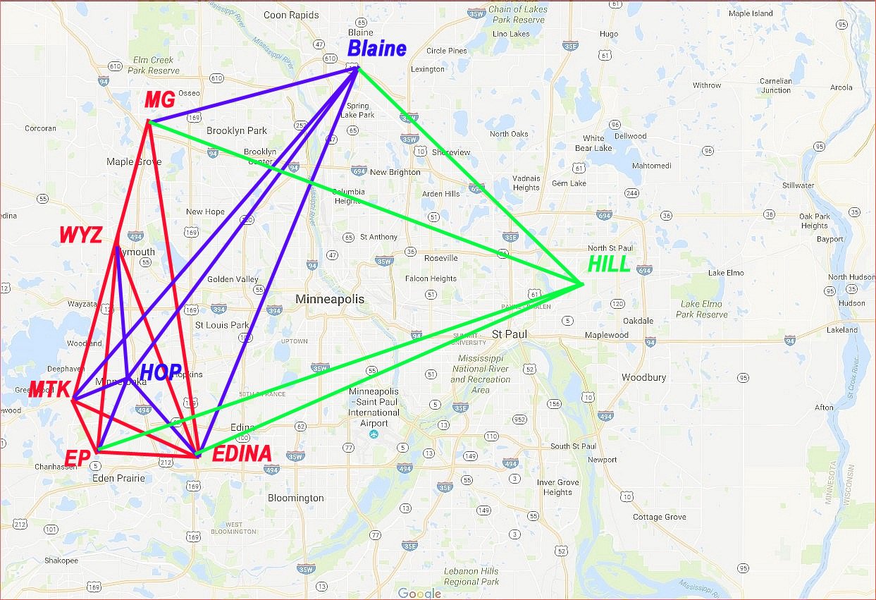
Figure 1 - Game network connections between teams.

One more clarification in nomenclature needs to be explained before diving into the numerical example, and that is the definition of a residual, denoted by the letter "little v". The residual v is defined as the difference between the observed value and its most probable value, i.e., it's the observed margin of victory (MOV) of a game minus its predicted MOV. In other words, it's the random error between what the theoretical model predicts and the God honest truth.

(Observed MOV)i - (Predicted MOV)i   =   vi                                                              (3-1)

Next, let's write out the observation equations. These equations relate each game MOV to the most probable values for each team's unknown rating values, i.e. in geospatial terms its unknown elevation and the residual errors in that game score.
Let
Teamh = Predicted rating of the home team.
Teama = Predicted rating of the away team.
MOVha(i) = Raw margin of victory of the i-th game between Teamh & Teama

Then equation 3-1 becomes
MOVha(i) - ( Teama - Teamh ) = vha(i) (3-2)
Rearranging so that MOVha(i) is on the right hand side of the equation with the residual Teama - Teamh = MOVha(i) + vha(i) (3-3)
Therefore the nine games in Table 1 and the single benchmark observation translates into
WYZ - EP = -6 + v1
EP - EDINA = -2 + v2
EDINA - MG = 1 + v3
MG - WYZ = 7 + v4
EP - MTK = 0 + v5
EDINA - MTK = 3 + v6
MTK - MG = -2 + v7
WYZ - MTK = -3 + v8
EDINA - WYZ = 6 + v9
EDINA = 1000 + V10

........................................................................ (3-4)

Rearranging once more so that the residuals are on the left-hand side of the equation, and squaring the residual yields:
v12 = (WYZ - EP + 6)2
v22 = (EP - EDINA + 2)2
v32 = (EDINA - MG - 1)2
v42 = (MG - WYZ - 7)2
v52 = (EP - MTK - 0)2
v62 = (EDINA - MTK - 3)2
v72 = (MTK - MG + 2)2
v82 = (WYZ - MTK + 3)2
v92 = (EDINA - WYZ - 6)2
V102 = ( EDINA - 1000)2

.................................................................. (3-5)

To express the condition of least squares, one must minimize the sum of the square of the residuals, meaning that this minimization condition is going to give us the best fitting solution to our model whether it is modeling a straight linear or a higher order polynomial. Let the game residual function G(v) be equal to the sum of the square of the residuals, we write:
G(v) = Σ( i =1 to n v2(i) ) = minimum (3-6)
in this example n = 10, the total number of observations, and expanded as
G(v) = v21 + v22 + v23 + v24 + v25 + v26 + v27 + v28 + v29 + v210 = minimum (3-7)
Substituting into equation 3-7 the values for the squared residuals in equation 3-5 the following game residual function is obtained:
G(v) = (WYZ - EP + 6)2 + (EP - EDINA + 2)2 + (EDINA - MG - 1)2 + (MG - WYZ - 7)2
+ (EP - MTK + 0)2 + (EDINA - MTK - 3)2 + (MTK - MG + 2)2 + (WYZ - MTK + 3)2
+ (EDINA - WYZ - 6)2 + (EDINA - 1000)2 = minimum (3-8)

The next step is to write out the partial derivatives of the game residual function G(v) shown in equation 3-8 with respect to each unknown rating variable, i.e. the rating value of each team in the network and set the resulting partial derivative equal to zero. Since we have five unknown (red) team rankings, these yield five normal equations. (Note: Although Edina is assigned a benchmark elevation of 1000.0, it is still considered an unknown in this set of equations).
= -2(EP - EDINA + 2) + 2(EDINA - MG - 1) + 2(EDINA - MTK -3)
+ 2(EDINA - WYZ - 6) + 2(EDINA - 1000) = 0 (3-9)

 =   -2(WYZ - EP + 6) + 2(EP - EDINA + 2)  +  2(EP- MTK)  =  0                       (3-10)


  =   -2(EDINA - MG - 1)  + 2(MG - WYZ - 7) - 2(MTK - MG + 2)  =  0             (3-11)


              =   -2(EP - MTK)  - 2(EDINA - MTK - 3)  +  2(MTK - MG + 2) 
                    - 2(WYZ - MTK + 3)  =  0                                                                              (3-12)   

              =   2(WYZ - EP + 6)  -  2(MG - WYZ - 7)  + 2(WYZ - MTK + 3)  
                 - 2(EDINA - WYZ - 6)  =  0                                                                               (3-13)          

Reducing the above normal equations 3-9 to 3-13 by dividing by a factor of two and collecting like terms yields equations 3-15 to 3-18, respectively:
+5 EDINA -1 EP -1 MG -1 MTK -1 WYZ = +1012 (3-14)
-1 EDINA +3 EP +0 MG -1 MTK -1 WYZ = +4 (3-15)
-1 EDINA +0 EP +3 MG -1 MTK -1 WYZ = +8 (3-16)
-1 EDINA -1 EP -1 MG +4 MTK -1 WYZ = -2 (3-17)
-1 EDINA -1 EP -1 MG -1 MTK +4 WYZ = -22 (3-18)

These five normal equations above (3-14 through 3-18) can be represented in matrix form where the left hand side contains the Normal Matrix (N) having 25 elements is arranged as a 5x5 square matrix and contains the coefficients of the unknowns. The N-matrix is also called the design matrix. The solution vector is a 5x1 column matrix containing five unknowns, and the right hand side is a 5x1 column matrix of constants that is composed of the observations. Let's examine the structure of the N-matrix. Notice that the diagonal elements are all positive integer numbers. Element [1,1] contains the number of observations connected to the EDINA team, elements [2,2], [3,3], [4,4] and [5,5] contain the number connections to EP, MG, MTK and WYZ teams respectively. Also notice elements [3,2] and [2,3] which both contain zeros and represents the fact that there are no direct connections between teams EP and MG, i.e. in our sample of games in Table 1 EP did not play against MG. The remaining off-diagonal elements are all the same value, being -1, indicating a single game connection between the ith row and jth column teams, respectively.
5 -1 -1 -1 -1
-1 3 0 -1 -1
-1 0 3 -1 -1
-1 -1 -1 4 -1
-1 -1 -1 -1 4
EDINA
EP
MG
MTK
WYZ
1012
+4
+8
-2
-22

5N5 = 5X1 = 5ATL1 =

Figure 2 - Normal Equations structure for red team network.

The general matrix notation for the complete system of equations and its solution are:
                       5N5     ∙     5X1          =                        5ATL1                                                (3-19)                                                      5N -15  ∙  5N5     ∙     5X1          =     5N -15    ∙    5ATL1                                                (3-20)
                  5I5           ∙      5X1          =     5N -15    ∙    5ATL1                                               (3-21)
                                         5X1          =      5N -15    ∙    5ATL1                                              (3-22)

1 1 1 1 1
1 22/15 17/15 6/5 6/5
1 17/15 22/15 6/5 6/5
1 6/5 6/5 7/5 6/5
1 6/5 6/5 6/5 7/5
1 0 0 0 0
0 1 0 0 0
0 0 1 0 0
0 0 0 1 0
0 0 0 0 1

Figure 3 - Inverse of the N-matrix for red team network. Figure 4 - Identity Matrix

Note that the Identity matrix I = N -1∙N. Solving for the above five reduced normal equations simultaneously yields the following adjusted rating values for each team (see Table 2).

Table 2 - Most probable values (MPV) of Team Quality for network of red teams
Team Computations MPV
EDINA = (1 x 1012) + (1 x 4) + (1 x 8) + (1 x -2) + (1 x -22) = 1000.000
EP = (1 x 1012) + (22/15 x 4) + (17/15 x 8) + (6/5 x -2) + (6/5 x -22) = 998.133
MG = (1 x 1012) + (17/15 x 4) + (22/15 x 8) + (6/5 x -2) + (6/5 x -22) = 999.467
MTK = (1 x 1012) + (6/5 x 4) + (6/5 x 8) + (7/5 x -2) + (6/5 x -22) = 997.200
WYZ = (1 x 1012) + (6/5 x 4) + (6/5 x 8) + (6/5 x -2) + (7/5 x -22) = 993.200

Based on this very small set of nine observations with four degrees of freedom (DOF = nine independent observations - five unknown variables), we see that EDINA has a slightly higher rating than both EP and MG by 1.867 and 0.533 of a goal, respectively. If this seems like a lot of work to do to calculate values by hand, even for a small network like this five station example, you are not in the minority. Fortunately, we can use matrix methods, software and computers to rapidly calculate values for a much larger network. We can describe the set of unweighted observation equations presented in equation 3-4 using the following matrix form:
obsAunk ∙ unkX1 = obsL1 + obsV1 (3-23)
obs equals the number of observations (number of games plus benchmarks)
unk equals the number of unknowns (number of teams in the league)
obsAunk is called the A-matrix, and contains the coefficients of the partial derivatives of the
observation equations as given in equation 3-3. It is a regular matrix with "obs"
rows and "unk" columns.

unkX1 is called the solution vector, and contains the most probable values to the team
rating profile. It is a column matrix with "unk" number of rows.
obsL1 is called the "L"-matrix, and contains the MOV observations for each game
corresponding to the row of the A-Matrix. It is a column matrix with "obs" rows.
obsV1 is called the "V"-matrix, and contains the residuals corresponding to each
observation equation in the A-matrix. It is a column matrix with "obs" rows.

Using matrix methods in least squares adjustments can vastly simplify the calculation process which also provides us with the tools we need later to evaluate the precision of the rating profile values. The previous example of the five red teams is now considered in matrix form. Let the A-matrix, X-matrix, L-matrix and V-matrix have the following values:
0 -1 0 0 1
-1 1 0 0 0
1 0 -1 0 0
0 0 1 0 -1
0 1 0 -1 0
1 0 0 -1 0
0 0 -1 1 0
0 0 0 -1 1
1 0 0 0 -1
1 0 0 0 0
-6
-2
1
7
0
3
-2
-3
6
1000
1.067
0.133
-0.467
-0.733
0.933
-0.200
-0.267
-1.000
0.800
0.000
EDINA
1000.0
EP
998.133
MG
999.467
MTK
997.200
WYZ
993.200

.

Recall equation 3-3 for a moment, [ Teama - Teamh = MOVha(i) + vha(i) ] and consider game #1 listed in Table 1. Substituting the most probable values into 3-3 that we previously calculated for both EP and WYZ, we calculate the residual value for that particular game to be: [ 993.200wyz - 998.133ep] + 6 = 1.067 = v1 (3-24)

Note: prior to the actual matrix solution, the Italicized values in the solution vector X and residual matrix V are not known. The least squares matrix solution proceeds as follows:

0 -1 0 0 1
-1 1 0 0 0
1 0 -1 0 0
0 0 1 0 -1
0 1 0 -1 0
1 0 0 -1 0
0 0 -1 1 0
0 0 0 -1 1
1 0 0 0 -1
1 0 0 0 0
0 -1 1 0 0 1 0 0 1 1
-1 1 0 0 1 0 0 0 0 0
0 0 -1 1 0 0 -1 0 0 0
0 0 0 0 -1 -1 1 -1 0 0
1 0 0 -1 0 0 0 1 -1 0

5 -1 -1 -1 -1
-1 3 0 -1 -1
-1 0 3 -1 -1
-1 -1 -1 4 -1
-1 -1 -1 -1 4

         = 

0 -1 1 0 0 1 0 0 1 1
-1 1 0 0 1 0 0 0 0 0
0 0 -1 1 0 0 -1 0 0 0
0 0 0 0 -1 -1 1 -1 0 0
1 0 0 -1 0 0 0 1 -1 0
-6
-2
1
7
0
3
-2
-3
6
1000
1012
+4
+8
-2
-22

Recall that the (ATA)-1 matrix is also known as the inverse of the N-matrix from Figure 3

1 1 1 1 1
1 22/15 17/15 6/5 6/5
1 17/15 22/15 6/5 6/5
1 6/5 6/5 7/5 6/5
1 6/5 6/5 6/5 7/5

Finally the most probable values are calculated as:

1 1 1 1 1
1 22/15 17/15 6/5 6/5
1 17/15 22/15 6/5 6/5
1 6/5 6/5 7/5 6/5
1 6/5 6/5 6/5 7/5
1012
+4
+8
-2
-22
1000.0
998.133
999.467
997.200
993.200

As a post-solution step, one should compute and plot the observation residuals to check for extreme values, either natural outliers or blunders in the data.

0 -1 0 0 1
-1 1 0 0 0
1 0 -1 0 0
0 0 1 0 -1
0 1 0 -1 0
1 0 0 -1 0
0 0 -1 1 0
0 0 0 -1 1
1 0 0 0 -1
1 0 0 0 0

1000.0
998.133
999.467
997.200
993.200
-4.933
-1.867
0.533
6.267
0.933
2.800
-2.267
-4.000
6.800
1000

To compute the residuals vector, we rearrange equation 3-23, which yields:

-4.933
-1.867
0.533
6.267
0.933
2.800
-2.267
-4.000
6.800
1000
-6
-2
1
7
0
3
-2
-3
6
1000
1.067
0.133
-0.467
-0.733
0.933
-0.200
-0.267
-1.000
0.800
0.000

A plot of the residuals versus the observed MOV values in the L-matrix shows no apparent outliers in the data and the pattern of white noise indicate a good fit to the observation model.

Recalling equation 3-6 [ G(v) = Σ( i =1 to n v2(i) ) = minimum ] , performing the summation yields G(v) = 4.533 we will use this value later in the discussion.

4 Discussion
So far we have learned a very powerful (and impartial) method to produce a rating scale that answers that nagging question that gets under the skin of every hockey fan, "Which teams are better than the others, and by how much?" Sounds like a Sesame Street jingle. We have partially answered the big question, but first we really do need to address yet another related question, and that is "What is the amount of uncertainty in this rating list that we have meticulously produced? The short answer to this is just to use the ratings as a predictive tool, and then compare the predicted game outcomes to the real deal. Simple enough? Well not quite, because the accuracy of your predictions is largely associated with the precision of your rating list. Figure 6 below illustrates the relationship between accuracy and precision.

Figure 6 - Accuracy vs. Precision
Without dragging the reader through a set of long theoretical proofs, let's just cut to the chase with regard to understanding how to recover precision information from the least squares method. Basically there are two parts to computing a value that describes the precision of a rating value for any given team. One part has to do with the measurement values and how close they are to the predicted model values. Ok you guessed it, the residuals. The second and equally important part of this has to do with the design of the network. In hockey terms, it has everything to do with who play's against whom? The physical geometric design of the network highly contributes to the achievable precision or lack there of in any given rating profile. Equation 4-1 is a rigorous formula to compute the variance for any individual team's rating value.
Sx2 = So2 ∙ (ATPA)-1 = So2 ∙ Q (4-1)
As previously stated, the variance (Sx2 ) is composed of two elements that are multiplied together. The first element is the square of So (pronounced "Sigma-naught") and is calculated using the following formula:
So = (4-2)
Where
p is the weight of an observation
v is the residual of an observation
n is the number of observations
DOF are the degrees of freedom in the system of normal equations that was solved

Let's apply these formulas to our example network of five red teams {Edina ... Wayzata}. First, we set p = 1.0 because we stated previously that the solution would employ equal weights. Therefore the numerator under the square root is equal to the game residual function G(v) = 4.533 Next the total degrees of freedom in the system (DOF) will be set to a value of four, which is computed as nine games minus five teams. Substitute values and reduce, we get
So = √ ( 4.533 / 4 ) = 1.0645
The second piece of information that we need to gather is found in the (ATPA)-1 matrix which is namely the inverse of the N-matrix (design matrix) denoted as N -1, and by convention is called the variance-covariance matrix, which is also denoted by the letter capital "Qxx". P is the weight matrix which we will ignore once more because for our special case, it is an identify matrix due to using equal weights set to 1.0 . The diagonal elements of the Q-matrix are what we are interested in, which correspond to each team in the network. By slightly changing the form of equation 4-1, the estimated standard deviation Sxi for any unknown (i.e. a team's quality rating) that was included in the solution to the normal equations, is expressed as:
Sxi = So ∙ (4-3)
Qxixi is the value of the diagonal element (located in ith row and column) of the Q-matrix.
Recall from our small network of five red teams, the diagonal elements are (high-lighted):
EDINA EP MG MTK WYZ
↓ ↓ ↓ ↓ ↓

1 1 1 1 1
1 22/15 17/15 6/5 6/5
1 17/15 22/15 6/5 6/5
1 6/5 6/5 7/5 6/5
1 6/5 6/5 6/5 7/5
←EDINA
←EP
Qxx = ←MG
←MTK
←WYZ

Therefore the uncertainty, in team EP rating value is Sep = (1.0645) x √(22/15) = 1.289
Qualifying team EP's rating value is expressed as 998.133 ± 1.289 . The standard deviation value for team MG is the same as EP because the two diagonal elements [2,2] and [3,3] are both 22/15, whereas teams MTK and WYZ would share the same value of Smtk = Swyz = ± 1.260, while the value for Sedina = ± 1.0645 . The average hockey fan might say, "Wow that's a huge range plus or minus 1.3 goals, what good does that do for us ... etc.". Fair point, but remember this is the results from only one game per team! The conventional wisdom among those that perform computerized hockey ratings is that one would like to see a minimum of five to seven games played per team before processing the game scores. Prior to the five or seven game milestone, the magnitude of the uncertainty is large enough that it's just not worthwhile to produce a meaningful rating profile. This is mainly due to the network design factor, ie., the value of the diagonal elements in the Q-matrix become significantly smaller as more and more interconnections are made between teams. To illustrate this concept, we added three more teams: HOP, BLAINE and HILL to the original five team network to form an eight team network. The game score data in Table 3 and Figure 1 show the additional network connections that were made, yielding a total of thirteen DOF's, more than tripling that of the original five team configuration. A new adjustment was computed, and the Qxx values corresponding to the diagonal elements are shown in Table 4. Excluding team EDINA because it was assigned as a control point (its Qxx value is equal to 1.0 and will not change numerically), we can examine the Qxx values of the remaining four red teams being EP, MG, MTK and WYZ. On average, the Qxx (diagonal element) values became smaller in magnitude by approximately 10% solely due to a stronger network design.
Table 3 - Game scores for an eight team network Table 4 - Qxx comparison

Game Away
Team Home
Team Score
Away Score
Home Score
Diff
1 WYZ EP 0 6 -6
2 EP EDINA 1 3 -2
3 EDINA MG 2 1 +1
4 MG WYZ 8 1 +7
5 EP MTK 0 0 0
6 EDINA MTK 4 1 +3
7 MTK MG 2 4 -2
8 WYZ MTK 1 4 -3
9 EDINA WYZ 6 0 +6
10 HOP EDINA 1 7 -6
11 HOP EP 0 3 -3
12 HOP MTK 0 2 -2
13 HOP WYZ 3 1 +2
14 BLAINE MG 1 1 0
15 BLAINE MTK 4 1 +3
16 BLAINE HOP 4 2 +2
17 BLAINE EDINA 0 4 -4
18 HILL BLAINE 4 4 0
19 HILL MG 2 1 +1
20 HILL EP 2 4 -2
21 HILL EDINA 1 3 -2
Team Qxx
(5 Teams) Qxx
(8 Teams)
% Δ
EDINA 1.0000 1.0000 -0-
EP 1.4667 1.3018 -11.24
MG 1.4667 1.3018 -11.24
MTK 1.4000 1.2724 -9.11
WYZ 1.4000 1.3031 -6.92
HOP 1.3031
BLAINE 1.3081
HILL 1.3465

The rate of change of the estimated standard deviation for the entire Minnesota Girls HS hockey league was tracked over a ten week period corresponding to the second half of the season and culminating with the week of the high school state tournament. Figure 7 below shows a family of trend lines, one for each week during this ten week period. Each trend line consists of a list of estimated standard deviations in ascending order of that week's MSHSL rating profile computed for the entire 120 girls teams in the league. The trend line for week 0 (zero) was generated from a least squares adjustment that contained games played up until December 10th, 2016 , approximately ten games per team. Subsequently, trend lines for weeks 1 through 10 were generated using the total cumulative number of games played up until the nominal end of that week's game schedule. The trend lines are non-linear in form, and gently slope upward from left to right. Clearly, as the season progressed and more and more games (interconnections) were played, the overall strength of the design matrix (N) increased such that each subsequent trend line shows a reduction (top to bottom) in the average magnitude of the estimate standard deviations. Additionally, the general slopes of the trend lines become flatter as the season progresses, i.e. the range of values becomes smaller from left to right. For example, the trend line range of week 0 starts at 1.1 and finishes at 1.5, while the range of week 10 is half that, starting at 0.6 and finishing at approximately 0.8 .

Figure 7 - Rate of change in estimated standard deviations weeks 0 to 10
There are three important pieces of information that we can derive out of Figure 7. First, the precisions of early to mid-season ratings are not as good as those later in the season, by approximately a factor of two. Secondly, one can assign a quantifiable precision number to the week by week rating profiles. For example, by the end of the season on week 10, the precision of the final rating profile ranges from 0.6 to 0.8 goals, depending upon the specific team. Thirdly, the week to week rate of improvement in precision is decreasing over the course of the season. We see this pattern by comparing the average difference between two subsequent trend lines. For example, the average difference between week 1 and week 0 is approximately 0.1, whereas the difference between week 10 and 9 is roughly one-tenth of that, approximately 0.01. The main reason for this is that most teams over the course of the season, end up replicating games against a few teams in their specific athletic conference, rather than playing new teams which as we know strengthens the overall network. Replication of games against a group of teams can either increase or decrease the magnitude of So depending upon the situation, thus directly impacting the estimated standard deviation. In the majority of the cases where two teams play each other more than once during the season, the two separate game MOV outcomes tend to be similar, thus reinforcing the solution model. In some cases though, one team may improve significantly over time with respect to the other, thus the two game outcomes can be quite different (or even reversed) causing So to increase due to larger residual values. This is part and parcel to the nature of sport teams, since the previous losing team is more motivated to play well to avoid a second loss to their rival. We can predict this behavior, but we cannot plan or count on it. But what is possible, is that we can optimize the design of the interconnecting network in order to achieve a desired level of precision. Since the estimated standard deviations are directly proportional to the Q-matrix, and the Q-matrix is simply the inverse of only the ATA matrix, we can perform simulations to optimize the strength of the entire network without knowing a single score! At last, those of us who perform team ratings usually have little influence on the game scheduling process, but if we did wouldn't this be useful information!
Finally, there are two concepts to cover before we can present a statistical method to answer our ultimate question; these concepts involve error propagation and the definition of an adjusted observation. Let's address the latter next. An adjusted observation denoted by the symbol î, is simply the actual game MOVi plus its residual value vi. For example, the adjusted MOV observation for the first game in Table 1 (WYZ @ EP) is -6.000 + 1.067 = -4.933 . This should look familiar because its exactly the save as the difference between the predicted quality ratings for each team, where WYZ - EP = 993.2 - 998.133 = -4.933 . The next important concept is the generalized law of propagation of variances, which is given by the following equation:
Σîî = A Σxx AT (4-4)
where î represents the adjusted MOV observations, Σîî the covariance matrix of the adjusted observations, A the coefficient matrix of the MOV observations, and Σxx the covariance matrix of the unknown parameters, i.e. the unknown parameters are the quality rating for each team. (Ghilani 2006) Recall that Σxx can be expressed as So2∙ Qxx , substituting into 4-4 yields:
Σîî = So2∙A Qxx AT (4-5)
where A Qxx AT = Qîî which is the cofactor matrix of the adjusted MOV's. That was a substantial piece of complicated terminology in one paragraph, so let's simplify it using our five red team network example by putting some actual numbers to these symbols. Substituting values into the A-matrix from page 12 and Qxx matrix from page 17, and So from page 16 yields the following equation for the estimated standard deviations in the adjusted MOV using matrix form:

0 -1 0 0 1
-1 1 0 0 0
1 0 -1 0 0
0 0 1 0 -1
0 1 0 -1 0
1 0 0 -1 0
0 0 -1 1 0
0 0 0 -1 1
1 0 0 0 -1
1 0 0 0 0

15 15 15 15 15
15 22 17 18 18
15 17 22 18 18
15 18 18 21 18
15 18 18 18 21

0 -1 1 0 0 1 0 0 1 1
-1 1 0 0 1 0 0 0 0 0
0 0 -1 1 0 0 -1 0 0 0
0 0 0 0 -1 -1 1 -1 0 0
1 0 0 -1 0 0 0 1 -1 0

Performing the necessary matrix multiplication steps in equation 4-6 results in:

6 -4 -1 -2 -3 0 -1 3 -3 0
-4 7 -2 -1 4 -3 1 0 -3 0
-1 -2 7 -4 1 3 4 0 3 0
-2 -1 -4 7 -1 0 -4 -3 3 0
-3 4 1 -1 7 3 -2 3 0 0
0 -3 3 0 3 6 -3 3 3 0
-1 1 4 -4 -2 -3 7 -3 3 0
3 0 0 -3 3 3 -3 6 -3 0
-3 -3 3 3 0 3 0 -3 6 0
0 0 0 0 0 0 0 0 0 15

The estimated standard deviation of an observation is calculated by computing the square root of the ith diagonal element of the Σîî covariance matrix corresponding to the desired game MOV. For example, in game No.6 listed in Table 1, EDINA beat MTK by a MOV equal to +3 goals. The corresponding element in the cofactor matrix is Qîî[6,6] thus the estimated margin of error (MOEΔ) at 68% confidence level of the adjusted MOV is
MOEΔedina-mtk = ± 1.0645 √ = ± 0.673 goals
In statistical lingo the concise meaning of the margin of error (MOEΔ) value above is that there is a 68% probability that the true value is within the range of ±0.673 goals of the adjusted MOV (î6 = Ɩ6 + v6 = 3.0 + 0.20 = 3.200 goals). Restated, the true value lies within the interval defined by the region 3.200 ± 0.673 goals [2.527 ↔ 3.873] with a 68% confidence level. At this point the average hockey fan is asking "What's so unique about a 68% confidence level?" Nothing special, except it just happens to correspond to the symmetric central portion under the Normal probability function defined by plus or minus one standard deviation on either side of the center line of the curve (its domain being -∞ to +∞). The width of the computed margin of error MOEΔ can be stretched for any probability level by using a multiplier defined by an appropriate t-value or z-value, depending upon how many degrees of freedom exists in the least squares solution of the network. The t distribution approaches the shape of the z distribution at very large DOF values. Perhaps, more appropriately we should use a 95% confidence level. The rational behind using the 95% level, is elegantly stated by Professor Emeritus Marty Triola as "The confidence level of 95% is most common because it provides a good balance between precision (as reflected in the width of the confidence interval) and reliability (as expressed by the confidence level)." (Triola 2015, p.320) Table 5 contains the most common confidence levels and their corresponding alpha (α), critical z-values, and t-values.
Table 5 - Confidence Levels.

Confidence
Level α Critical Values

Z α/2 (3000 dof)
t α/2 (4 dof)
t α/2
68% 0.32 1.000 1.000
90% 0.10 1.645 1.645 2.134
95% 0.05 1.960 1.960 2.776
99% 0.01 2.575 2.576 4.604

On closer examination of the matrix multiplication steps involved in solving equation 4-6, we see that a more efficient algorithm can be employed that will yield the same results for the desired diagonal element of the Qîî matrix.  Instead of using the entire A-matrix, we only need the row of coefficients corresponding to the diagonal element of interest.  Furthermore, only three elements from the Qxx matrix are required.  These three elements are the two diagonal elements corresponding to each team in the observation equation, and the covariance element between these two teams.  Since a row of the A -matrix will also always contain a single +1 corresponding to the away team, and a single -1 corresponding to the home team, and remaining elements are 0 (because only two teams can play in one game!) the equation to calculate the confidence interval and margin of error for an adjusted observation reduces to the following:

    C.I. î  =  [ MOVi  +  vi ]  ±                                     (4-8)

Where
MOVi is the game margin of victory between the away team and home team.
vi is the computed residual for the ith game
Qjj is the jth diagonal element of the Qxx matrix corresponding to the Home team
Qkk is the kth diagonal element of the Qxx matrix corresponding to the Away team
Qjk is the jth row and kth column off-diagonal element of the Qxx matrix
tα/2 is the student t-value for the desired confidence level at a given DOF
So is the standard deviation of unit weight of the LS adjustment (eqn. 4-2, p.16)
For example, using game no.6 once more, the C.I. and margin of error (MOE) using equation 4-8 is computed as: [ (3.0 + 0.200) ± (1.0)∙ ] = [ 3.2 ± 0.673 ]
In geospatial terms, another important use for equation 4-8 is to compute the margin of error for observations that were never made. In the case of sports teams, we can do the same for games never played. Recall that in Table 1, teams EP and MG never played each other (in this example) thus we can use 4-8 and the predicted quality rating profile values to construct a 95% confidence interval for a hypothetical game MOV between these two teams. Substituting values and performing the math steps yields:
[(MG - EP) ± MOEΔ] = [(999.467 - 998.133) ± (2.776) ]
95% C.I. = [(1.334) ± (2.413)] = [ -1.1 < MOVmg-ep < +3.7 ] (rounded)
The interpretation of the above calculation is: "We are 95% confident that the interval from -1.1 to +3.7 actually does contain the true MOV between MG and EP if they were to play a hockey game against one another". Notice that the computed CI contains within its interval the value of zero, and extends slightly beyond -1. Based on this early season rating profile, this is suggesting that either team might just win the ice hockey contest. In fact, on Nov 26th, MG beat EP by a score of 2 to 0, yielding a MOV = +2 which is well within the compute 95% CI above. Looking at the on-line post-game stat sheet it appears that the game was a closer contest than the 2-0 final score indicates. MG had scored its two goals (1 power play and the other even strength) during the second period, although EP had actually out-shot MG 14 to 10 during the same period. By the end of the game, EP had the edge on MG in total shots on goal (SOG) 27 to 25, plus EP had fewer penalty infractions 6 min versus 10 min. Perhaps MG had the better goalie that day which was just enough that EP couldn't find a way to put the puck in the back of the net. Regardless, it was a close contest as the 95% CI suggests.
To compute whether one team is statistically better than another at any given confidence level, the condition that the predicted MOV between the two teams must be greater than the MOEΔ, that is the MOVi - MOEΔ > 0. By rewriting equation 4-8 such that MOVi = MOEΔ and solving for tα/2 we now have a test statistic to judge against a claim. Let the null hypothesis and the alternative hypothesis be:
Ho : Teamj = Teamk
H1 : Teamj ≠ Teamk (4-9)
Let the test statistic equal
tα/2 = (4-10)
Where
= predicted MOV between the jth and kth teams
Qjj is the jth diagonal element of the Qxx matrix corresponding to the Home team
Qkk is the kth diagonal element of the Qxx matrix corresponding to the Away team
Qjk is the jth row and kth column off-diagonal element of the Qxx matrix
So is the standard deviation of unit weight of the LS adjustment (eqn. 4-2, p.16)

After the end of the Girls MSHSL post-season state tournament, a boastful claim had been made by a renowned hockey pundit that the Blake HS team was clearly a better team than the Edina HS team.  Both teams were ranked No.1 in their respective class designations during the entire regular season, Blake in class (single) A and Edina in class (double) AA, and both teams ended up winning the championship game in their respective divisions at the state tournament held at the Xcel Energy Center in downtown Saint Paul, MN.  Towards the end of the regular season schedule the Blake did indeed beat Edina by one goal (2 to 1) in a very close, hard fought contest in which Edina heavily out-shot Blake by a margin of 24 to 11 SOG.  That game was the only loss of the season for Edina, where as Blake had loss two games plus tied one game to three different teams that Edina had previously soundly beaten.  Also Edina had tied with Breck HS, which had loss to Blake.  Through-out the post-season sectional and state tournament play-offs, Edina most certainly faced a much tougher and impressive (AA) strength of schedule than Blake's (A). Each team's final season win-loss-tie records were Edina (28-1-1) and Blake (27-2-1). 

Example:
Using a 95% confidence level (α = 0.05), test who is the better team; Edina or Blake and by how much? Construct the 95% confidence interval for a hypothetic MOV between these two teams played at a neutral site.
Ho : TeamEdina = TeamBlake
H1 : TeamEdina ≠ TeamBlake

We extracted the following parameter values from the computed rating profile for week no.10.
Given
DOF = 3000 (3283 games - 283 teams = 3000)
So = 2.421 (standard deviation of unit weight from LSqr solution)
TeamEdina = 1001.7913 (predicted quality rating week 10)
TeamBlake = 1000.4260 (predicted quality rating week 10)
MOVE-B = +1.3653 (predicted margin of victory in goals by TeamEdina)
QxxEdina = 0.061650892 (variance TeamEdina : diagonal element of Qxx)
QxxBlake = 0.067469169 (variance TeamBlake : diagonal element of Qxx)
QxxE↔B = 0.031110952 (covariance Edina vs. Blake: off-diagonal element of Qxx)

Substituting the above parameter values into equation 4-10 yields a student t-value of 2.180 . From Table 5 the critical t-value at the 95% confidence level (using 3000 DOFs) is 1.960. Comparing the test statistic to the critical t-value we find that ttest > tcrit (2.180 > 1.96) . Another way of looking at this comparison is to find the P-value of the test statistic. Using a Ti-84 calculator, our t-score of 2.180 corresponds to a P-value of 0.029335 which is smaller than our selected alpha level of 0.05. In other words, the test statistic value falls inside the tail region defined by the critical t-value. Therefore when P is low (0.029335 < 0.05) the Ho must go! (Triola 2015) There is sufficient evidence to reject the Ho, meaning that the proclamation by the local hockey pundit claiming that the Blake team is a better quality team than Edina seems to be a lot of huff and puff, i.e. it's a false claim. The 95% CI for a neutral site game is calculate as CI = (1001.7913 - 1000.4260) ± (1.96)∙(2.421)∙√(0.0668981) = (1.3653) ± (1.227), or rounded as [ 0.14 < MOV < 2.59] . We are 95% confident that the true MOV for a neutral site game between Edina and Blake girls teams will be contained in the interval from 0.14 to 2.59 in favor of Edina.

5 Remarks
Emotions can run high when it comes to most anything concerning the beloved sport of high school ice hockey in Minnesota, the self-proclaimed "State of Hockey" in America. The supporters and follower of the girls high school programs tend to be a bit thinner-skinned than their counter parts on the boys side of the equation, so when it comes to ranking and rating players and teams, there are a few sacred cows skating on the ice rinks that the public dare not scrutinize too closely without fear of retribution. By employing the methodology of least squares to develop a sound rating profile, one can avoid the ill-effects of human/political bias when it comes to evaluating which groups of teams are succeeding, struggling or otherwise. Additionally, once a reliable rating profile is created and its precision qualified, its powerful content can be extended to identify and evaluate overlooked individual talent to help promote those players whom may not have had the benefit of being handed the golden baton at a younger age. Elaborating on rigorous numerical and statistical methods such as presented in this paper is key to achieving these goals with the hope of providing more opportunities to well deserving players and teams.

6 Conclusion
At the onset of writing this paper, the intention was to provide the audience (i.e. your average hockey fan, player, coach or scout) with a practical appreciation of what the nuts and bolts of a rating profile are, and how they can and should be used to benefit the players and teams involved in the particular league of interest. On after thought, the material presented most likely requires the reader to have had at least one introductory statistics course, plus an intermediate level math course to fully understand the "How-To" matrix methods laid out to perform and apply the calculations. With that said, I hopefully believe that after reading this article, one will take away with them one important point about the nature of these ubiquitous rating profiles that they see in society, which is that they question where the data came from, what process did it follow and by whom it was produced, and finally what is the inherit precision of its content. The understanding that comes from this lesson in math and statistics won't ever rid us of the emotional aspects of ranking and rating our favorite sports team, but it should make us all a bit more harmonious when we interact with each other. So the next time your not-so-favorite buddy makes the claim that his/her team is better than yours, now you have a way to statistically test that claim (equation 4-10), and just maybe provide your good friend with a more humbling viewpoint. Go Hornets!

7 Glossary

Confidence Level
the probability that the value of a parameter falls within a specified range of values.

Critical t-value
in hypothesis testing, a critical value is a point on the test distribution that is compared to the test statistic to determine whether to reject the null hypothesis.

Geospatial
relating to or denoting data that is associated with a particular location.

Ho - Null Hypothesis
(in a statistical test) the hypothesis that there is no significant difference between specified populations, any observed difference being due to sampling or experimental error.

Ha - Alternative Hypothesis
is contrary to the null hypothesis. It is usually taken to be that the observations are the result of a real effect (with some amount of chance variation superposed).

Margin of Error
is usually defined as the radius (or half the width) of the confidence interval for that statistic.

Nomenclature
the body or system of names in a particular field.

Normal equations
any of a set of simultaneous equations involving experimental unknowns and derived from a larger number of observation equations in the course of least-squares adjustment of observations.

Partial derivative
a derivative of a function of two or more variables with respect to one variable, the other(s) being treated as constant.

P-value
the calculated probability, is the probability of finding the observed, or more extreme, results when the null hypothesis (H 0) of a study question is true.

8 References

Bassett, Gilbert W. Jr. (1996), Predicting the Final Score. Manuscript, University of Illinois at Chicago, Dept of Economics, Web. < http://citeseerx.ist.psu.edu/viewdoc/download?doi
=10.1.1.195.2676&rep=rep1&type=pdf>

Brezinski, Claude and Dominique Tounès (2014), André-Louis Cholesky (1875-1918) Mathematician, Topographer and Army Officer. Birkhäuser, Basel, IX+ 311 pages.

Ghilani, Charles and Paul R. Wolf (2006), Adjustment Computations: spatial data analysis. Wiley, 4th ed., 611 pages.

Massey, Kenneth. (1997), Statistical Models Applied to the Rating of Sports Teams. Masters's Thesis. Bluefield College. < http://www.masseyratings.com/theory/massey97.pdf>

Stefani, R. T. (1977), “Football and Basketball Predictions using Least Squares,”
IEEE Transactions on Systems, Man, and Cybernetics. 7, 117–120.

Triola, Mario F. (2015), Essentials of Statistics. Pearson, 5th ed. 670 pages.