DIY - Linear Forecasting with Python

profitgenerator (68)in #mathematics • 7 years ago (edited)

So let’s do some more interesting things with Python. As I said previously I am all for people learning stuff for themselves and not have to rely on other’s. Do it yourself is really the slogan of liberty if you think about it.

So why would you rely on “experts” when you can just analyze data yourself with basic statistical tools. I have said many times, Linux is like a God sent-gift, and combined with the Python programming language, it really empowers people beyond imagination to do and learn anything with it that your computer can support. It’s like a (semi) user-friendly direct control over your computers computing power, which is what computers are meant to be, so you can make your computer calculate anything you want.

Why would you stick to a closed-source OS where you have to purchase stuff for 100-400$, instead with this setup you can do it all for free, and do it all yourself, not relying on anyone else. It’s freedom.

Linear Forecasting

So forecasting data is a complex big subject but we will start with the basics which is linear forecasting. Linear forecasting only works on linear data. Linear data means that the data has a constant variance, homoskedastic data.

Linear forecasting is really the absolute basic stuff, so we have the given data:
1,2,3,4,5,x

What will x be? If you guessed 6, then you are correct.

So basically we are just forecasting the n+1 datapoint for a dataset of n values where x usually represents the random variable.

The way this is done is you just take the average of the differences starting from 2, the dataset must be at least n=2 size. So subtract the 2-1, 3-2,4-3,5-4, and then take the average of them, since it’s always 1, the average is 1. Then just add the difference to the last n datapoint to get the n+1 value.

Since the difference is constant, it’s enough if you take the difference of x_n-x_n-1 points, the last one minus the one before, to get the difference, since it won’t change, it will be 1 in this example, and then add that to the last one. Although this is not recommended for other datasets where the difference changes.

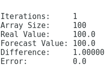
So we can forecast n+1,n+2,n+3,… all the way to infinity since this dataset will never change, it counts 1 by 1 towards infinity thus we can forecast every single future point with a 100% accuracy. But this would be too easy, in reality you will never come by a series like this in practice, especially not in finance, so this is just theoretical.

I wrote a quick Python script to emulate this. We have an array of a size of 1000, basically counting from 1-100 by 1, and we have to forecast what comes after 99. Well using the method described above, we take the differences across all pairs starting from 2:

arraysize=1000 # MIN 2

def fillarray_linear():
   asum=0.0
   for i in range(arraysize):
      asum=asum+1.0
      ARRAY[i]=asum

def linear_forecast_diff():
   fillarray_linear()
   f_diff=0.0
   for i in range(1,arraysize): # calculate f_diff
      f_diff=f_diff + (ARRAY[i]-ARRAY[i-1])

   f_diff/=(arraysize-1)
   return f_diff

And then we verify the forecasted value against the actual future value (of course we are always working on past data in theory, so the n+1 data is the n_th data, shifted back 1 units in the past, if we want to backtest the forecasting strategy):

def verification():
   f_diff=linear_forecast_diff()
   last_real=ARRAY[arraysize-1]
   last_forecast=ARRAY[arraysize-2]+f_diff
   error=abs(math.log(last_forecast/last_real))   
   return last_real,last_forecast,f_diff,error

Now as described in the previous article, I really like using LN() based errors, not Root Mean Square and crap like that, that is biased like hell. In fact since I mostly use this for finance, like working on cryptocurrency markets, it makes sense to use the LN() error, instead of additive errors.

To give you an idea:

If the price forecast mismatches from 10000$ to 8000$ that is like a 2000 error, but it’s only a potential 20% loss.
If the price forecast mismatches from 1$ to 0.80$ that is only a 0.2 error, but it’s still a 20% loss

So as you can see the additive error model sucks, especially for finance, we only work with ratios here since the profits and losses are in ratios related to the buy/sell price. So in the example above the 2000 error is nonsense since it represents the same loss as the 0.2 error. Thus in LN() form that is an error of 0.223143551 in both cases, and since the LN() function is additive, while raw percentages are not, it’s the ultimate way to calculate errors.

Furthermore we take the ABS() value of the error, so if we are just buying and selling without shorting then we should make a difference between + error and – error, since overestimating the price is still a profit, but we shouldn’t.

I mean it’s not like the function has any idea whether we are going to buy or short, so we must not discriminate between profits and losses, from an error standpoint it’s the same. We missed the target, we missed the target, that’s it.

Essentially we could divide it by 2, to only represent the “loss side” while ignoring the “profit side”, but it doesn’t even matter. It’s just a number, not necessarily like a predefined unit like meters or inches, it’s just a number, and if we use it this way, the only thing that matters is that it’s as close to 0 as possible.

Linear Forecasting with Entropy

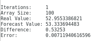
So the first example is easy, a completely predictable time series, in this example we are going to add some entropy to it, basically making the co-variance high. So in the previous example the co-variance was 0, in this example it will not be 0, thus the difference will change, but it’s still a homoskedastic series since the covariance is bound.

In this example I am going to fill the array with RANDOM(0.01,1) numbers, but since they are bound it’s still possible to forecast this to some extent.

def fillarray_random():
   asum=0.0
   for i in range(arraysize):
      asum=asum+random.uniform(0.01,1)
      ARRAY[i]=asum


def linear_forecast_diff():
   fillarray_random()
   f_diff=0.0
   for i in range(1,arraysize): # calculate f_diff
      f_diff=f_diff + (ARRAY[i]-ARRAY[i-1])

   f_diff/=(arraysize-1)
   return f_diff


def verification():
   f_diff=linear_forecast_diff()
   last_real=ARRAY[arraysize-1]
   last_forecast=ARRAY[arraysize-2]+f_diff
   error=abs(math.log(last_forecast/last_real))   
   return last_real,last_forecast,f_diff,error

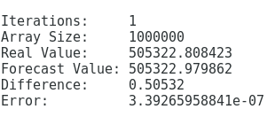
To increase our accuracy we set the array size to 1,000,000 so that we will have a larger sample to draw differences from, to see what is going on there.

The difference should be (1+0.01)/2=0.505 which is the expected value of the random number generator but we don’t know that,remember, so we are trying to estimate that from a large sample of data!

See it’s pretty darn close now, the expected value is 0.505 and we got 0.50532. So that is only a potential loss of 0.0000339%. If we could forecast the BTC/USD market with this accuracy it would be cool, but no so fast.

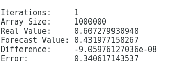
So as you can see, a trending data has an expected value if we would have used a stationary data without a trend:

def fillarray_random():
   for i in range(arraysize):
      ARRAY[i]=random.uniform(0.01,1)

Then the difference trends towards 0, this is because in a stationary model, the expected value is 0, that is no change, since it’s basically just a distribution between the 2 limits but no change, this means a constant mean, a constant variance and a constant covariance.

Conclusion

Thats the basics, of course this is only for homoskedastic markets, and it’s linear forecasting, most of the time it’s never this easy, and we will get into more complicated modeling and forecasting methods in the future. I have put together the entire script which is available here.

Download Full Script Here

So you can play around with linear forecasting, it hardly has any use case unless it’s like a trivial example like counting things. However in the random case above, where the variance is changing but the mean is constant, well that is similar to weather forecasting and things like that.

But for finance, neither the mean, nor the variance nor covariance is constant, so that is a heteroskedastic model, where things like ARIMAX(1,1,1) or SARIMAX(1,1,1) can be used. Later on those.

In fact I have wrote plenty posts about those already in the past:

Sources: