So Many Graphic Novels, So Much to Manage - Inventory Part 2

Continuing from this post: https://steemit.com/computers/@phoenix32/so-many-graphic-novels-so-much-to-manage-inventory-part-1

Making the initial spreadsheet for the Inventory was actually not that challenging. Expanding it to accommodate numerous Authors that have written and Issues that are contained within each graphic novel actually proved to be a smart move, even if the main page was static - it was actually easier to have separate cells for each entry as opposed to cramming all of the information into a single cell for each category. In retrospect, I feel that cramming all of the authors and issues into their own cells was just sloppy. It also created massive misalignments in the displaying of the cells - text had to be horizontally centered in all cells, and that created a weird "<>" type of appearance, since Series and Title were singular, Issues and Authors could be extensive, and Publisher was almost always singular.

Spreading it out made for an easier view of the data in terms of spacing - and with wider screens these days, I could still see most of what I needed to see. Of course, there is the horizontal scrolling, but I found that preferable to the variations in cell heights. I could also maintain a constant for column widths by utilizing the largest size for all of the columns in the Issues group and making that the norm; same for the Authors group. Now I have consistency - YAY!

The breakdown of the columns is as follows:

• A - BookID
• B - Series_Name
• C - Title
• D - Publisher
• E - Type
• F - ISBN
• G-U - Issues
• V-AO - Authors
• AP - Shelf #
• AQ - Status
• AR-AX - Character_Tags

Some context for a few of these columns... BookID is for database-type entries, as originally I wanted to import the sheet into Microsoft Access. Everything needs a unique identifier, but now it is a terrific sorting tool. When sorting alphabetically, there is a disparity for certain books. As I was trying to be true to the actual titles, I will again cite the "War Games" arc from Batman (Volume 1). The prelude is "War Drums," and the trilogy is "War Games Act One: Outbreak," "War Games Act Two: Tides," and "War Games Act Three: Endgame," and the prologue book is "War Crimes." Spreadsheet alphabetical order would place them out of sequence:

• War Crimes
• War Drums
• War Games Act One: Outbreak
• War Games Act Three: Endgame
• War Games Act Two: Tides

This does not work for sequencing of the books, and even if I used numbers instead of the words for the numbering for "War Games," that does not fix "War Crimes" and "War Drums." So when I sort the document, I do so first by Series, then by BookID, and lastly by Title.

Granted, that 3rd sort category of "Title" might be unnecessary - OK, OK, it really is unnecessary - but I do that to emphasize the point. Plus, it has helped me sort out some typos in along the way, and when you're dealing with over 1,000 books, there is a great chance that a typo has been made at one point or another. I've caught quite a few over the years (in fact, I just had some difficulty with this very sentence... heh...), and there is little doubt that I would find more.

I've actually reset the numbering system a couple of times, however, as I have purchased books that would not fall into any proper sequencing. Recently, I purchased reprints of "Batman: Prodigal" and " Batman: Troika." Both of which, thankfully, fall nicely into sequence with the Knightfall Trilogy, so it looks like this when I sort and filter:

Speaking of filters...

The lovely little "\ /" at the right of Row 1 are for filtering. I love filtering. It is great for quick searches for a single columns or for Series and Title. It helps to remove from view books that are in the way. So when I was searching for the Knightfall Trilogy, Prodigal, and Troika, I did a filter by Title:

It helps to know almost exactly what you are looking for when you filter; otherwise, you can just use more filters.

Aside from the "Graphic_Novels" sheet, the workbook consists of other sheets, all of which are cross-linked to "Graphic_Novels", as it is the source sheet.

• Form Responses 1
• Publisher_Breakdown
• Counts
• Character_Query
• Issues_Query
• Author_Query
• Publishers

Let's start with the easy one: Form Responses 1. I use a Google Form to input the information for each book, and then I copy-and-paste the information from there into the "Graphic_Novels" sheet.

Next up is "Publishers". This is a source sheet, and is necessary due to having multiple publishers for at least 3 different titles in my collection.

I used a few simple commands for some of the cells:


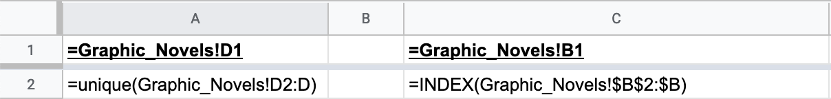
The formulae in cells A1 and C1 are basic commands, linking to cells B1 and D1 on the "Graphic_Novels" sheet, respectively. If I change the values on either of those cells on "Graphic_Novels", then the linked cells on "Publishers" will also change. Pretty straightforward, right? Next is in cell A2. Please note - you're going to want to keep all of column A blank, as the formula that I used in A2 can span from a single row up to filling the entire column, depending on the source. I used the "UNIQUE" function and applied to the range of column D on Graphic_Novels, but with a restriction. Had I used "=UNIQUE(Graphic_Novels!D:D)" as the command, it would have included cell D1, which is the header row, so I limited the function to start at D2 and include the entirety of the column below it. "UNIQUE" does not alphabetize the items in the list, it just grabs the information and lists items only once, no matter how many times they appear in the list.

I used a similar function in column C with the "INDEX" function. This lists every item in the given range, again skipping the header row and starting at row 2. This listed the Series_Name of ever book in the collection. While this makes for some redundancy - OK, a crap-ton of redundancy - this is again due to the Series that fall under multiple publishers. While I could have started from A1 and C1 and used the whole range of Graphic_Novels!D:D and Graphic_Novels!B:B, I wanted to make certain to keep the header rows on the "Publisher" sheet separate as well. I prefer some level of fine-tune control in my work, just enough to make certain that I am not sorting things improperly.

Next, I wanted to take the uniquely separated values of the publishers and reorganize them in a row instead of a column. The "TRANSPOSE" command did this nicely, so long as I placed the value in cell D1 and kept the rest of the row blank. Granted, I could have used an imbedded formula "=TRANSPOSE(UNIQUE(Graphic_Novels!D2:D))" which would have done the job nicely, however, I also needed the list in column A in the first place, so why make the sheet work harder than it has to work.
Here's a small sample of the results of the array that is contained by column C and row 1:

And this is an example of the contents of cell D2: "=IF(AND(Graphic_Novels!$B2=$C2,Graphic_Novels!$D2=D$1),$C2,"")"
Oh, yeah, let's break this down a bit...

• "Graphic_Novels!$B2=$C2" is an evaluative command, with the "$" used to demarcate a constant value for "Graphic_Novels" column B and for column C of the current sheet. This is to compare the Series_Name and make certain it matches.
• "Graphic_Novels!$D2=D$1" is the same kind of command, making certain that the Publisher value matches. The D$1 means that, as I shift from left to right, the column value will change in relative to its position in other columns, but the row will remain constant at row 1.
• Both are linked by an "AND" command: which means that both of these have to be true values, otherwise there will be an error.
• In order to avoid having an error message, I used an "IF" command which will either give out the value of cell C2 in the event that the "AND" command comes back true, or the "" means that the value of cell C2 will be left blank in the event that the "AND" command comes back false.

I populated the sheet by copy-and-pasting the command to the length and breadth of the remainder of the sheet with no need for formulaic editing. This whole set up is essential for the "Publisher_Breakdown" sheet in order to provide certain calculations.

I would love to have used the "TRANSPOSE" function, but the use of merged cells on row 1 makes it impossible, as "TRANSPOSE" uses the actual cells, starting (in this case) from G1 and onward. However, my grouping and merging is in clumps of four: G1-J1, K1-N1, O1-R1, S1-V1, et cetera, and this was essential, seeing as I grouped four columns together for each Publisher.

The first column ("G") provides a count for the Series by that Publisher, the second column ("H") is the name of the Series, the third column ("I") is the number of Titles in that particular Series, and the fourth and last column ("J") is the percentage of the of the Series to the entire collection. The italicized Title (and respective information) in Row 2 is the biggest title for the Publisher. In my collection, Batman (Volume 1) edges out Amazing Spider-Man (1963) by just a couple of books, and together they make up close to 10% of my collection.

Yeah, I know, I spoke of the "family member" characters - Nightwing, Robin, Scarlet Spider, Venom, blah blah blah - as being essential to my collection, and that is still true. Most of the Batman (Volume 1) books that I own are ones such as "Prodigal," "Troika," "War Games," and more that have those characters contained in the epics. My ASM (1963) has some of my favorites, such as Scarlet Spider/Ben Reilly, Venom/any-random-host... I'm going to just let that rest right here and move along...

The way that I populated the cells was based on the data from the "Publishers" sheet:

The "header row" starts in the left-most cell, G1, so all of the formulae reflect back to that.

• Cell G3: =IF(H3="","",1)
• Cell G4: =IF(H4="","",G3+1); this is subsequent for column G
• Cell H3: =IF(G1="","",UNIQUE(FILTER(Publishers!D2:D,Publishers!D2:D<>""))); an imbedded formula, first I used the "FILTER" function with a caveat to ignore blanks, putting into a "UNIQUE" to avoid duplications, and then the "IF" function to avoid unsightly "N/A" outputs and instead leave fields blank, so it looks pretty.
• Cell I3: =IF(H3="","",COUNTIF(Publishers!D$2:D,H3)); dependent upon cell H3, again with the "IF" function to make it pretty, the "COUNTIF" function would scan the given range on the "Publishers" sheet and provide the number of times that it would appear based on the value in cell H3.
• Cell J3: =IF(H3="","",I3/$B$2); this gives the percentage of the Series against the entire collection, with a static reference to cell B2, held in place with the twin "$", one for column and one for row.

The other four-column groupings were identical, utilizing the respective "header row" cells. I framed the four-column groupings out with borders to separate the data, and (of course) "froze" the "header row" so that there was some organization and reference as you scroll down. Also, as you can see from the screenshot below, one of the biggest reasons for having the "Publishers" sheet to sort the data is because of titles such as "Danger Girl," as she was published by both Wildstorm and IDW. The same holds true for "Transformers," a Marvel once held and now IDW currently holds rights to the Series.

The big deal on this sheet is, for me, the conditional formatting that I used all the way to the left of the sheet. Cell A2 contains the formula: =IF(MAX(Graphic_Novels!A2:A)=$B$2,"OK!","Oops..."). This means that A2 will read "OK!" or "Oops..." if the value of cell B2 is equal in value to the maximum value from the range of column A2:A on the "Graphic_Novels" sheet. The conditional format looks like this:

Translated into the King's English - since A2 will only have 1 of 2 values, the text would be bold in either case, although it would be red if A2 read "Oops..." and it would be green if A2 read "OK!"

Cells B2, C2, and D2 are all dependent on other numerical values:

• B2: =MAX(Graphic_Novels!A2:A); this looks for the maximum value in column A2:A on the "Graphic_Novels" sheet - this is the largest BookID.
• C2: =MAX(Counts!D2:D); this looks for the maximum value in column D2:D on the "Counts" sheet - this is the largest ID# of the Series list.
• D2: =ROUND(SUM(D3:D),4); strictly "local" to this sheet, the "SUM" function adds up the entire range (column D3:D) and the "ROUND" function delimits the percentage show to a length of 4 - 1,0,0, and %. Admittedly, that is not the most appropriate definition of this function, but it is getting the job done for the moment.
• Each of these cells has a distinct conditional format:

B2:

C2:

D2:

There are conditional formats for the the ranges of B3:B, C3:C, and D3:D as well.
B3:B uses an "is equal to" value, each formula adapted to the particulars of the publisher four-column grouping:

• B3: =sum(I3:I)
• B4: =sum(M3:M)
• B5: =sum(Q3:Q)

C3:C uses a Custom formula, as it has multiple conditions that must be met in order for the formatting to be applied:

• C3: =AND(SUM(I3:I)=B3,ROUND(SUM(J3:J),4)=D3)
• C4: =AND(SUM(M3:M)=B4,ROUND(SUM(N3:N),4)=D4)
• C5: =AND(SUM(Q3:Q)=B5,ROUND(SUM(R3:R),4)=D5)

D3:D uses an "is equal to" value, each formula adapted to the particulars of the publisher four-column grouping:

• D3: =ROUND(sum(J3:J),4)
• D4: =ROUND(sum(N3:N),4)
• D5: =ROUND(sum(R3:R),4)

Here's what things would look like if there was an error somewhere:

I even applied a conditional format to the "Graphic_Novels" sheet, column A1:A1201, a Custom formula: =countif(A:A,A1)>1. This will scan the entire column for duplicate entries, ensuring that each number is a unique BookID. Here's a sample of what happens when an ID is duplicated:

At this point, this formula needs to be manually adjusted as more rows are added to the "Graphic_Novels" sheet, so user beware! It really is a simple matter of adjusting the range on the conditions.

So that covers the publishers, some of the numbers, and the conditional formatting! There will be a Part 3 coming very soon, in which I'll cover the various Query sheets. Thanks for reading!