image source

Data science and Machine learning have become buzzwords that swept the world by storm. They say that data scientist is one of the sexiest job in the 21st century, and machine learning online courses can be found easily online, focusing on fancy machine learning models such as random forest, state vector machine and neural networks. However, machine learning and choosing models is just a small part of the data science pipeline.

This is part 4 of a 4 part tutorial which provides a step-by-step guide in addressing a data science problem with machine learning, using the complete data science pipeline and python pandas and sklearn as a tool, to analyse and covert data into useful information that can be used by a business. The previous parts of the tutorial can be found here:

Part 1
Part 2
Part 3

In this tutorial, I will be using a dataset that is publicly available which can be found in the following link:

https://archive.ics.uci.edu/ml/datasets/BlogFeedback

Note that this was used in an interview question for a data scientist position at a certain financial institute. The question was: whether this data is useful. It’s a vague question, but it is often what businesses face – they don’t really have any particular application in mind. The actual value of data need to be discovered.

The final tutorial will be covering the last step in the pipeline: Trying to improve the model, and evaluating the result in real life and draw conclusions from it.

Recap

We have applied our first machine learning model, ensemble model known as gradient boosting, using scikit-learn. The model is saved as clf, and from the cross validation data we obtained two different metrics, the confusion matrix, and the AUC ROC score, both of which are giving a reasonable result quantitatively. But how does it correspond to usefulness of the model in real life, and can we make this model better?

Interpreting the model in real life

Before we can improve a machine learning model, we need to understand what the model means or how the model is used in real life. A lot of metrics are in fact trade-offs with each other, so the one that we need to optimise depends on how we use the model. For example, it is well known that recall is a trade off with precision: the more sample that a model predict is positive, the more true positive samples will be captured (higher recall), while at the same time the proportion of false positive will increase (lower precision), and vice versa. Therefore, one cannot optimise both, and which one to optimise is solely based on the application. For an application associated with detecting breast cancer, we would want to optimise recall, as the consequence of missing a true case of cancer is potentially fatal compared to a much less consequential false positive case. On the other hand, for an application associated with detecting habitable exoplanets, precision should be optimised, as we do not necessary need to capture all habitable planets, but false positives would incur heavy costs in dead end explorations.

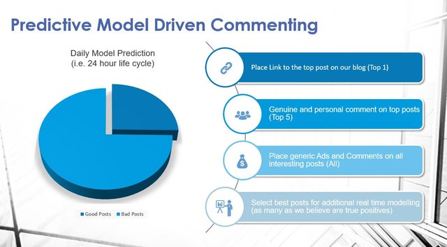
For our case here, it turns out that we want to optimise neither. That's because if we look at our application, neither of these are measures of real success. The real success is how much user exposure has increased by using this model. I can think of four different ways to use the output of this model, within the framework of social media advertising:

1. Select 5 of the posts we are most confident with (for becoming popular), and gain exposures by placing meaningful comments on these posts
2. Select the 1 post that we are most confident with and reblog or retweet
3. Place generic comments or Ads under all posts predicted to be popular.
4. Use the predicted post to do further real-time analysis. This requires selecting those that we believe are true positives

These are presented in the slide below.

To measure the total user that we are exposed to, we can measure the number of comments that the selected posts captured. For example, if the 5 posts that we selected to comment on ended up having 1500 comments in total, we would have been exposed to more users and hence more successful than if the 5 posts selected ended up having only 500 comments in total. We can then create metrics for assessing the model, according to the four conditions above, by writing a custom function:

import pandas as pd
import numpy as np
def compare_comment_count(target, predictions, pred_prob, entries = 50):
                df = pd.DataFrame(columns = ['comments', 'important_pred', 'pred_prob'])
                df.comments = target
                df.important_pred = predictions
                df.pred_prob = pred_prob
                df_predicted = df[df['important_pred'] == True]
                pred_indices = df_predicted.index
                chosen_posts = np.random.choice(pred_indices, entries, replace = False)
                total_count = df.loc[chosen_posts, 'comments'].sum()
                max_count = df.sort_values('comments', ascending = False).iloc[0:entries].comments.sum()
                rank_count = df_predicted.sort_values('pred_prob', ascending = False).iloc[0:entries].comments.sum()
                random_count = df.loc[np.random.choice(df.index, entries, replace = False), 'comments'].sum()
        return total_count, max_count, random_count, rank_count

This function takes in target, which is the ground truth, and prediction, the corresponding class prediction by the model, pred_prob, the confidence the model has that the prediction is true (i.e. class probability), and entries is the number of posts we want to select, which for the four criteria above, would be 5, 1, all posts, and 22% of the posts respectively.

The function return four values – total_count, which is the total number of comments captured by randomly chosen posts from those predicted by the model to be good; max_count, which is the number of comments that we can capture if we know a priori which posts are the most successful (this is used as a reference); rank_count, which is the number of comments captured if we rank all the positive prediction by class probability, i.e. taking the top posts that the model thinks is the most likely to be correct; and random_count, which is the number of comments captured if the posts were chosen randomly without prediction. A few interesting notes in terms of the code. First, note the sort_value() to sort a dataframe using a particular column, such as ‘comments’ or ‘pred_prob’. Also note the “.” notation for both calling dataframe functions and assessing columns of a dataframe. So by using iloc[0:entries].comments.sum() we are summing the comments column of the top entries number of rows.

Thus, to compare each of the cases required in the slide above, we can have the following script for example, for selecting 5 posts for meaningful comments:

test_proba = clf.predict_proba(X_test)
y_pred = clf.predict(X_test)
pred_count, max_count, random_count, rank_count = compare_comment_count(df_test.target_reg, y_pred, test_proba[:,1], entries = 5)
print('Comments Captured for take 5 post')
print('Random 5 posts with no modelling: ', random_count)
print('Random 5 from posts predicted to be good: ', pred_count)
print('Top 5 posts from posts predicted to be good: ', rank_count)
print('Maximum capture if we know which 5 posts are the best: ', max_count)

Note that the test data X_test was loaded from a small part of the test data set (data from the first half of Feburary 2012), where the rest of the test data will be used later for the final evaluation step. Please see previous tutorial for the processing for the test data. Also note how the class probability can be easily obtained using predict_proba(). Running the above script will result in the following:

The data shows that by applying the model and ranking the class probability, we can increase the comments captured by a whooping 50 times. Although it still fall short of the maximum comments captured possible, it is still a big achievement that you would be comfortable enough to sell to the executives.

Improving the model

There are a number of ways to further improve a machine learning model performance. The best option is to get more data if possible. The more data you have, the more likely you will be able to get a model that generalises to real data well, simply because you sample distribution gets closer to the real distribution if you have more data points. Of course, getting more real data is not always possible, and we could, as we demonstrated in the last tutorial, use bootstrapping to generate more data. However, since these duplicate data point really contains the same information, it can only get us so far. Getting more real data is always better.

Another way to improve the model is to combine different models. That is, apply a number of models to the same data set, then take a weighted average of the predictions given by these models. This is an ensemble method known as stacking. It works because statistically, each model would have different samples being predicted incorrectly, and therefore, if we take a weighted average of the prediction for one data point, we will be more likely to obtain the correct prediction. Stacking works best with models that are of a completely different type. Here, we will be using two other models, random forest, and k nearest neighbour algorithms. To simplify the scripts, I have written a function that train different models, depends on what model is specified:

from sklearn.ensemble import RandomForestClassifier
from sklearn.ensemble import GradientBoostingClassifier
from sklearn.neighbors import KNeighborsClassifier
def fit_and_predict(X, Y, X_test, Y_test, method):
        if method == "GBC":
                clf = GradientBoostingClassifier(learning_rate = 0.01, n_estimators = 500)
        elif method == "RF":
                clf = RandomForestClassifier(n_estimators = 1000)
        elif method == "knn":
                clf = KNeighborsClassifier(n_neighbors = 50)
        clf.fit(X, Y)
        test_proba = clf.predict_proba(X_test)
        y_pred = clf.predict(X_test)
        return clf, test_proba, y_pred

This function essentially takes in the training data X, Y and test data X_test, Y_test, and create a model depending on the specified method. In particular, if method = ‘GBC’ it will train a Gradient Boosted Classifier with 500 trees; if method = ‘RF’ it will train a Random Forest model with 1000 trees, and if method = ‘knn’ it will train a k-nearest neightbour classifier with k = 50. For each model, it will use the test data to get a set of class predictions (y_pred) and the corresponding class probability (test_proba). To combine the three models, we then use the following script:

clf_gbc, test_proba_gbc, y_pred_gbc = fit_and_predict(X_train, Y_train, X_test, Y_test, "GBC")
clf_rf, test_proba_rf, y_pred_rf = fit_and_predict(X_train, Y_train, X_test, Y_test, "RF")
clf_knn, test_proba_knn, y_pred_knn = fit_and_predict(X_train, Y_train, X_test, Y_test, "knn")
y_pred = ((test_proba_gbc[:,1] + test_proba_rf[:,1] + test_proba_knn[:,1]) > 1.8) & ((test_proba_gbc[:,0] + test_proba_rf[:,0] + test_proba_knn[:,0]) < 1.2) 
y_pred_proba = (test_proba_gbc[:,1] + test_proba_rf[:,1] + test_proba_knn[:,1])/3
total_count_combined, max_count, random_count, rank_count_combined = compare_comment_count(df_test.target_reg, y_pred, y_pred_proba, entries = 5)
print('Comments Captured for take 5 post')
print('Random 5 posts with no modelling: ', random_count)
print('Random 5 from posts predicted to be good: ', total_count_combined)
print('Top 5 posts from posts predicted to be good: ', rank_count_combined)
print('Maximum capture if we know which 5 posts are the best: ', max_count)

Note how we produce the prediction by combined the results from the three models using a weighted average of the class probability. In particular, a majority voting (i.e. looking at the class prediction from the three models and take the most common prediction) is equivalent to the sum of class probability for positive class to be > 1.5, and sum of class probability for negative class to be < 1.5. By changing this threshold we can tune the output of the combined model. For the combined class probability (for ranking purpose), we can just simply average the class probability of the three classes. Here is the result:

It doesn’t look like this method had improved the model by a lot. This probably mean that the gradient boosted classifier is already doing very well that combining other models with it does not improve its performance.

Final Evaluation

To perform the final evaluation, we need to realise that in real life, the model would be applied in a day-by-day basis, i.e. a 24 hour cycle as presented in the slide above. To use the test data, we would therefore load the test data in a day to day basis. Fortunately, that is how the data was formatted, that data from each day was stored in a separate folder. A function can be written as follows:

def evaluate_model(df_val, model):
        precision = 0.22    
        X_val = df_val.drop(['target_reg', 'target_clf'], axis = 1)     
        y_pred = model.predict(X_val)
        test_proba = model.predict_proba(X_val)[:,1]
        p_count = np.count_nonzero(y_pred)     
        if p_count < 5:
                entries = p_count
        else: 
                entries = 5
        top_one_tuple = compare_comment_count(df_val.target_reg, y_pred, test_proba, entries = 1)
        top_five_tuple = compare_comment_count(df_val.target_reg, y_pred, test_proba, entries = entries)
        all_positive_tuple = compare_comment_count(df_val.target_reg, y_pred, test_proba, entries = p_count)
        df_val['test_proba'] = test_proba
        df_val['y_pred'] = y_pred
        pred_tp = df_val.sort_values('test_proba', ascending = False).iloc[0:int(p_count*precision)].target_clf.sum()
        actual_tp = p_count*precision
        random_select = df_val.loc[np.random.choice(df_val.index, int(p_count*precision), replace = False), 'target_clf'].sum()
        random_select_p = df_val.loc[np.random.choice(df_val[df_val.y_pred == True].index, int(p_count*precision), replace = False), 'target_clf'].sum()
        precision_tuple = (random_select_p, actual_tp, random_select, pred_tp)
        return np.array(top_one_tuple), np.array(top_five_tuple), np.array(all_positive_tuple), np.array(precision_tuple)

which generate the result tuples top_one_tuple for selecting only 1 post, top_five_tuple for selecting only 5 posts, all_positive_tuple for selecting all positive posts, and precision_tuple for selected the top 22% (the precision determined from the last tutorial). Note that there is the complication that the number of positive post per day may be less than 5, and when that happens the top_five_tuple result is essentially the same as the all_positive_tuple. We need two more functions. The first one to load each test file:

def load_daily_validation(filename, name_list_final):
        df_test = pd.read_csv(filename, header = None, names = name_list_final)
        df_test = process_days(df_test)
        name_list10 = ['parents', 'parent_min', 'parent_max', 'parent_avg']
        name_list1 = []
        for i in range(50,60,1):
                 name_list1.append('mean_'+ str(i))
                name_list1.append('stdev_'+ str(i))
                name_list1.append('min_'+ str(i))
                name_list1.append('max_'+ str(i))
                name_list1.append('median_'+ str(i))
        df_test['target_clf'] = df_test.target_reg > 50
        df_test.drop(name_list1, axis = 1, inplace = True)
        df_test.drop(name_list10, axis = 1, inplace = True)
        return df_test

Please refer to the first tutorial and third tutorial for the column names of the table specified by name_list_final and the columns that are actually used in the machine learning model. Here, we are dropping all columns that have not been used in the machine learning model. Additionally, another function is written for evaluating and accumulating the daily comment captured:

def evaluate_model_all_files(validation_filelist, name_list_final, model):
        top_one = np.zeros(4)
        top_five = np.zeros(4)
        all_pos = np.zeros(4)
        prec_pos = np.zeros(4)
        for filename in validation_filelist:
                df_val = load_daily_validation(filename, name_list_final)
                df_val.Day_P = lb.transform(df_val.Day_P)
                df_val.Day_B = lb.transform(df_val.Day_B)
                array_one, array_five, array_all, array_prec = evaluate_model(df_val, model)
                top_one = top_one + array_one
                top_five = top_five + array_five
                all_pos = all_pos + array_all
                prec_pos = prec_pos + array_prec   
        return top_one, top_five, all_pos, prec_pos

Finally, we can execute the above functions to obtain the performance of the model:

validation_filelist = []
for filename in os.listdir('.'):
    if 'test' in filename:
        if (filename.split('.')[1] == '03'):
            validation_filelist.append(filename)
        elif ((filename.split('.')[1] == '02') and (int(filename.split('.')[2]) >= 16)):
            validation_filelist.append(filename)   
model_results = evaluate_model_all_files(validation_filelist, name_list_final, clf_gbc)
print('Final Results')
print('Top 1 post- Random:', model_results[0][2], ' Ranked Model: ', model_results[0][3], 'Max: ', model_results[0][1])
print('Top 5 posts- Random:', model_results[1][2], ' Ranked Model: ', model_results[1][3], 'Max: ', model_results[1][1])
print('All posts- Random:', model_results[2][2], ' Ranked Model: ', model_results[2][3], 'Max: ', model_results[2][1])
print('Precision posts- Random:', model_results[3][2], ' Ranked Model: ', model_results[3][3], 'Max: ', model_results[3][1])

Results shown below:

Comparing the results between random selection and a ranked model, it can be concluded that the model had improved the number of comments captured at least 10 times (although still only 50 - 60% of the maximum number of comments captured).

Presenting the Results

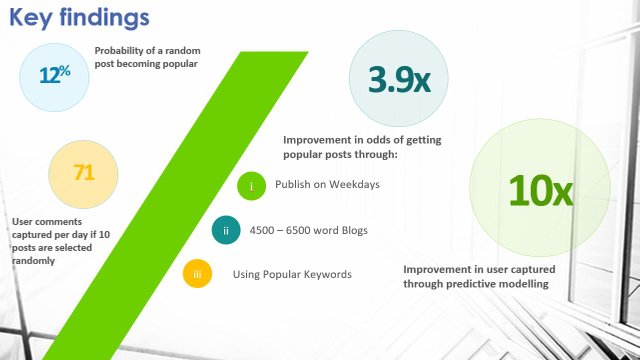
The final step of a data science problem is to draw conclusions that is tied to problem at hand. For our case here, the question was whether the data is useful enough that we should purchase it. Of course, the answer is yes. However, how do we sell this idea to the management? We need to highlight our findings. Recall from the previous tutorials, our findings include:

1. Using the data we can statistically improve the success rate of a blogpost our department wrote by using guidelines involving word counts, posting day etc
2. Using the data we can form a predictive model which increases our user exposure by capturing a higher number of comments.

We can present this conclusion in a more eye-catching way by adding in some numbers. For example, comparing with the success of a random post, we have determined that we can increase the rate of success by 3.9 times (from tutorial 2). In this tutorial, it was determined above that using the best model, we can capture 10 times more comments compare to randomly selecting a post. These are pretty strong numbers and is exactly what upper management want to see. We can present these using a slide in an eye-catching way:

So we have come to the end of our data science problem. In the four tutorials we have went through the data science pipeline, from loading and inspecting and processing of the data, basic statistical analysis, formulation and training of a machine learning model, and the interpretation of the model to draw conclusions. Note that this is a general pipeline that is application to any data science problem that you may have. I hope this tutorial series have been helpful for you.

---

Posted on Utopian.io - Rewarding Open Source Contributors

---