Step by step guide to Data Science with Python Pandas and sklearn #1: Understanding, Loading and Cleaning of Data

Data science and Machine learning has become buzzwords that swept the world by storm. They say that data scientist is one of the sexiest job in the 21st century, and machine learning online courses can be found easily online, focusing on fancy machine learning models such as random forest, state vector machine and neural networks. However, machine learning and choosing models is just a small part of the data science pipeline.

This is part 1 of a 4 part tutorial which provides a step-by-step guide in addressing a data science problem with machine learning, using the complete data science pipeline and python pandas and sklearn as a tool, to analyse and covert data into useful information that can be used by a business.

In this tutorial, I will be using a dataset that is publicly available which can be found in the following link:

https://archive.ics.uci.edu/ml/datasets/BlogFeedback

Note that this was used in an interview question for a data scientist position at a certain financial institute. The question was: whether this data is useful. It’s a vague question, but it is often what businesses face – they don’t really have any particular application in mind. The actual value of data need to be discovered.

The first tutorial will be covering the first steps in the pipeline: Understanding the data, Loading the data, and cleaning the data.

Understanding the Data

This dataset contain data extracted from blog posts. One thing about this data set is that it is a labelled dataset, which means that we know the meaning of each column, which would dramatically help us in using this data correctly. According to the website, the meaning of each column is as follows:

This data originates from blog posts. The raw HTML-documents of the blog posts were crawled and processed. The prediction task associated with the data is the prediction of the number of comments in the upcoming 24 hours. In order to simulate this situation, we choose a basetime (in the past) and select the blog posts that were published at most 72 hours before the selected base date/time. Then, we calculate all the features of the selected blog posts from the information that was available at the basetime, therefore each instance corresponds to a blog post. The target is the number of comments that the blog post received in the next 24 hours relative to the basetime.

1...50:
Average, standard deviation, min, max and median of the Attributes 51...60 for the source of the current blog post. With source we mean the blog on which the post appeared. For example, myblog.blog.org would be the source of the post myblog.blog.org/post_2010_09_10
51: Total number of comments before basetime
52: Number of comments in the last 24 hours before the basetime
53: Let T1 denote the datetime 48 hours before basetime,
Let T2 denote the datetime 24 hours before basetime.
This attribute is the number of comments in the time period between T1 and T2
54: Number of comments in the first 24 hours after the publication of the blog post, but before basetime
55: The difference of Attribute 52 and Attribute 53
56...60:
The same features as the attributes 51...55, but features 56...60 refer to the number of links (trackbacks), while features 51...55 refer to the number of comments.
61: The length of time between the publication of the blog post and basetime
62: The length of the blog post
63...262:
The 200 bag of words features for 200 frequent words of the text of the blog post
263...269: binary indicator features (0 or 1) for the weekday (Monday...Sunday) of the basetime
270...276: binary indicator features (0 or 1) for the weekday (Monday...Sunday) of the date of publication of the blog post
277: Number of parent pages: we consider a blog post P as a parent of blog post B, if B is a reply (trackback) to blog post P.
278...280: Minimum, maximum, average number of comments that the parents received
281: The target: the number of comments in the next 24 hours (relative to basetime)

For any dataset, it is important to first understand what the data represents before diving deep into the actual data. Let’s therefore study the description. From the description of the dataset above, we can see that each row of data was collected at a basetime (Note that the actual basetime is not recorded in the data). And data from all blogposts that was published at most 72 hours before the base time was recorded. These data include for example, number of comments, number of link backs, over 24, 48hr and 72hr time periods before the base time, words contained in the posts, length of posts, day at which the post was published, etc. The data was designed to be used to predict the number of comments a post would receive in the next 24 hours, and hence, being labelled data, we are actually given this number in the target column by assuming we are currently at the basetime.

Loading the Data

So let’s look at the dataset. In Python, one of the most useful tools for data processing is the Pandas package. More details of the pandas package can be found here. If you have Anaconda or Spyder, Pandas should already been installed. Note that Pandas build on Numpy, which is also already installed with Anaconda or Spyder. Otherwise, you would need to install both Numpy and Pandas.

Assuming that you have pandas installed, we can continue. First, import pandas into your python module.

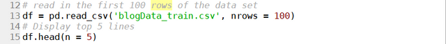
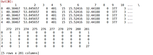
Next, we use the read_csv() command to load the data into a dataframe. Because data files could be extremely large, we will be careful here and first only load in the first 100 rows to have a look at what the data is like, i.e. nrows = 100. The function returns a dataframe, which is the main datatype used in pandas. It is essentially a table with rows and columns, and have special functions allowing data manipulation within the table. We will be using different dataframe functions in the rest of the tutorials. For example, to view the dataframe, one could use the head function which display the first n number of rows in the table. By default n is 5. A similar function tail let you view the last n rows of the data:

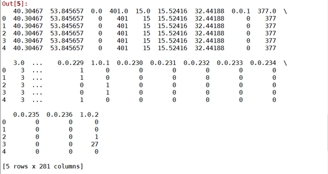
It can be seen that the dataframe has 281 rows as expected. Another thing to notice is that the column names are all numbers. This tells us that in fact, the data file does not have any headers. We will be addressing it later. The next step would be to probe how many rows the file has, as this would determine whether we can process the table as a whole, or if we could view it with some other software such as excel to gain more insights into the data. Apart from judging from the file size, one thing that I find useful is to only read the first column of the whole file. This will minimise the memory used. You can specify the columns that you want to read as a list in the read_csv function using the usecols parameter, remembering that the first column is indexed as 0. We can then probe the number of rows by using len(df):

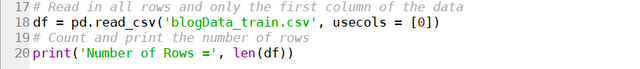
The number of rows in this file is only 52396. This is quite small by the data science standard. We can therefore safely load the whole data set into python in one go.

Before we do that, however, let’s go back to the issue of headers. In Pandas, one of the most powerful thing is you could refer to a column by its header name. This is convenient as it makes the code more readable, and less likely to lose track of which column of data is being processed. In this case here, since the file doesn’t actually have headers, it is useful to create headers, according to what the data is. read_csv() allows you to specify the name of the headers, again in a list, using the names parameter. You should also explicitly set the header parameter to None to tell the function that the data does not have any headers. So for example, you could do the following:

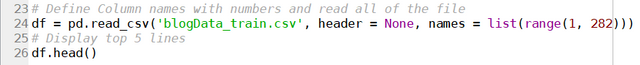
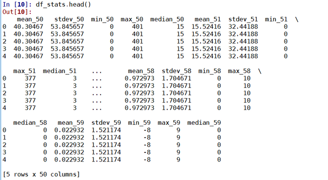
Which would read in the data with columns names ‘1’, ‘2’, ‘3’ … ‘281’, which of course, is not very useful. I would also argue that because these data can be grouped into different types (eg. number of comments, day of week, etc), it might be easier to read different sets of columns in as different dataframes. So this is what we will do here. For example, to read in the first 50 columns, which are the different statistics of columns 51 – 60, we can use the following code:

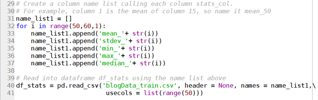
Remembering that usecols can be used to read in specific columns. We can check our success using head():

Similarly we can group the day of the week in which the blogpost was posted into a single dataframe:

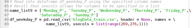
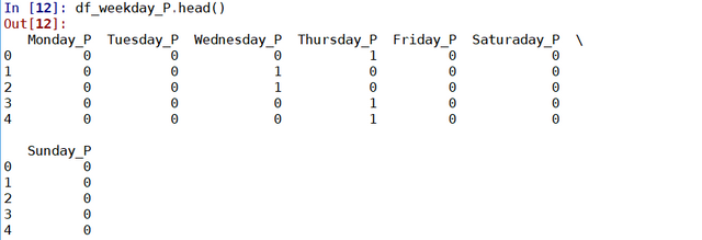
Note how for this dataframe, the data are 0 and 1. 1 if the day of the week corresponds to the column.

For this set of data, we can group the data into a number of dataframes as follows:
df_stats: Site Stats Data (columns 1 – 50)
df_total_comment: Total comment over 72hr (column 51)
df_prev_comments: Comment history data (columns 51 – 55)
df_prev_trackback: Link history data (columns 56 – 60)
df_time: Basetime - publish time (column 61)
df_length: Length of Blogpost (column 62)
df_bow: Bag of word data (column 63 – 262)
df_weekday_B: Basetime day of week (column 263 – 269)
df_weekday_P: Publish day of week (column 270 – 276)
df_parents: Parent data (column 277 – 280)
df_target: comments next 24hrs (column 281)

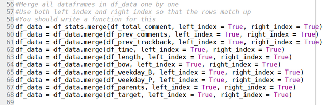
This would simplify the data analysis which I will show in the next tutorial. You can always combine these dataframes back into a single dataframe using the merge() function, using both left_index and right_index to match up the rows:

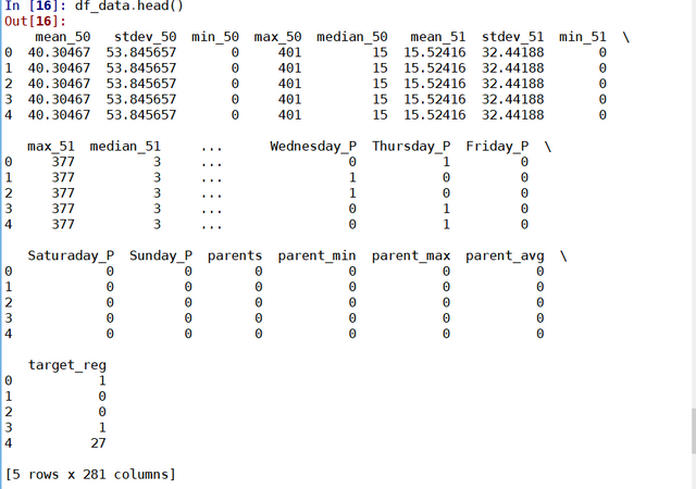
Again, use head() to confirm that everything is fine:

Cleaning the data

Now that the data is loaded into python, it is time to check the data and do some cleaning up. One of the things that you might want to do is to see if there are any missing data in the data set. This can be done using the isnull() function:

Which essentially sums up all the true and false values that is returned from the isnull() function. So the answer is greater than 0, then somewhere in the data set there is data is missing. In this case, there is no missing data. Alternatively, one can directly remove rows with missing data (if so wished) by directly calling the dropna() function:

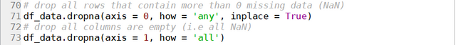
Note the keyword Inplace can be specified to be True to drop the rows/columns directly from the dataframe. Otherwise the function would return a new dataframe with the rows/columns dropped. Use shape() (a numpy function) to check the dimension of the processed table:

The number of rows (1st number) and columns (second number) is exactly the same as before, so there weren't any rows and columns that were dropped.

Looking at the day-of-the-week data, we can see that both df_weekday_B and df_weekday_P are using 7 columns to represent which day of the week it is. It may be easier to represent this with one single column that specify actual day of the week, rather than giving each day of the week a flag column.

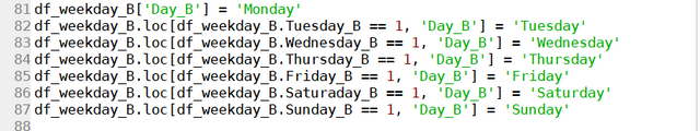
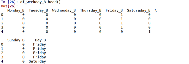
We can combine this into a single column by first creating a new column ‘Day_B’ in the df_weekday_B table, and set the default value as ‘Monday’. Next, we set the rows in the ‘Day_B’ to ‘Tuesday’ , ‘Wednesday’, ‘ Thursday’ etc when the corresponding flag is set. We do this by using the df.loc(row_function, column_function) which addresses the locations in the dataframe df where the row satisfy the row function and column satisfy the column function. In this case here, we look at say the Tuesday_B column, pluck out rows that have flag set to 1, and set the Day_B column of that row to ‘Tuesday’. Check the labels are correct again using head()

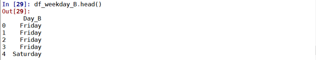
One can then finally drop all the flags column, and the table is left with one single column that contains the day-of-week information.


This can be repeated for df_weekday_P table as well.

The data is now loaded and ready to be analysed. This will be covered in the next part of the tutorial.

---

Posted on Utopian.io - Rewarding Open Source Contributors

---