How to calculate convolution of two signals | Scilab Tutorial
What Will I Learn?
- How to calculate convolution of two discrete-time signals
- How to use Scilab to obtain an approximation of Convolution of two continuous signals.
- How to define some special discrete and continuous signals regularly used in Signals and Systems learning. We'll do it on the fly.
Requirements
- Basic programming knowledge.
- Convolution mathematical operation knowledge.
- Scilab version 5.5.2 or higher.
Difficulty
- Basic
Tutorial Contents
Finally, I decided to make a tutorial about Convolution, since is quite difficult to find examples and very good tutorials (even made in Matlab) about this mathematical operation. I want you to learn the details about using the function
convin order to obtain very good results.
Convolution
Convolution is a mathematical operation whose applications are mostly in areas like Systems and Signal Processing, Physics and Engineering. Also, it’s a basic topic in engineering study programs, therefore if you are immersed in the engineering world, this tutorial will be useful for you.
Convolution operation of two discrete-time signals is defined as follow:

Convolution of two continuous-time signals is defined as follow:

Scilab provides several commands to perform convolution, nevertheless, each one has its own specialty, for example,convol uses Fast Fourier Transform, conv2 is used to work with two-dimensional arrays and frequently used in Image Processing. We’re going to use command conv.
Command conv is used to work with one-dimensional arrays and allows to handle the length of the result. Check its syntax
C= conv(x, y, “string”)
Where x and y are the vectors (Our signals) in question. The third argument is optional and allows to handle the dimension of the result, C. For example, writing full, which is the default value, will make the dimensions of the result are size(x)+size(y)+1and writing same will make the dimensions of the result are the same as those of x. We’re going to use same to obtain more illustrative results.
Discrete-time Convolution.
Discrete-time convolution is quite easy to perform with Scilab. Probably, defining the signals could be the challenge.
Let’s convolve the following signals
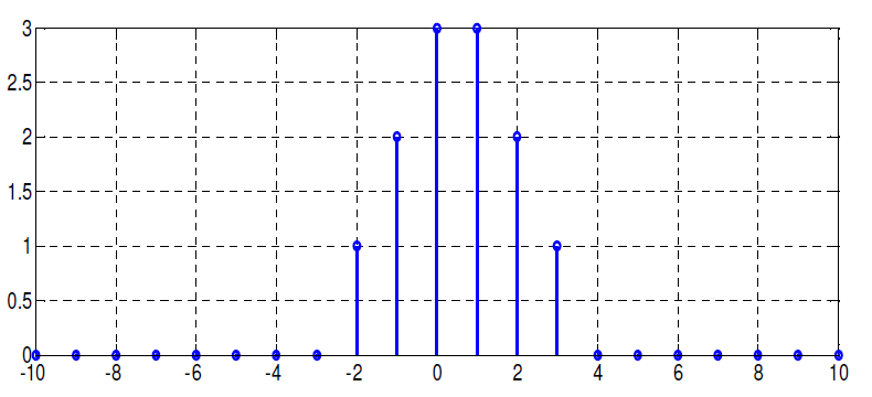

- The first step is defining the signals.
First, declare a discrete-time vector from -10 to 10, it will have 21 samples, you can check that in the Variable Browser.
There are many ways to construct the signal shown in figure 3, although I like the following way
 cond1= n>=-2 & n<=0;
cond2= n>=1 & n<=3;
x=0*n;
x(cond1)=[1 2 3];
x(cond2)=[3 2 1];
plot2d3(n,x);
After running the previous code segment you’ll get

Note that x(cond1) is a section of vector xof size three samples, therefore you can use the next syntaxes to get the same result
x(9:11)=[1 2 3];
or
x([9 10 11])=[1 2 3];
On the other hand, I’ve used function plot2d3 to plot x vs n instead plot2d, in order to get the curves plotted using vertical bars. This function is the equivalent of function stem (Matlab).
For the signal of figure 4 you can proceed in this way:
zo=zeros(1,9);
zo(4:6)=-1;
zo(7:9)=1;
z=zeros(1,21);
z(1:9)=zo;
z(10:18)=zo;
plot2d3(n,z);
The function zero(m, n) returns a (m,n) matrix of zeros, therefore zero(1,n) returns a row vector of zeros with n samples.
The result is shown in figure 6.

- Once your signals are ready you can proceed to the convolution step.
As I said, let’s use functionconvto convolve x[n] and z[n].
As I said, let’s use function conv to convolve x[n] and z[n].
C=conv(x,z,”same”);
plot2d3(n,C)
Take a look at the result.

You may want a grid in your figure. Matlab provides the command grid on but it doesn’t exist in Scilab, nevertheless it can be replaced by
set(gca(),"grid",[1 1])
Remember that if you leave the shape field empty, the dimensions of the result will be
size(x)+size(y)+1 therefore the previous code will become
C=conv(x,z);
plot2d3(-20:20,C)
set(gca(),"grid",[1 1]) // grid on
This is the new result

Finally, note that discrete-time convolution is easy, however continuous-time convolution is not. In fact, it’s technically impossible to do the convolution of two continuous-time signals with Scilab or any other software since computer data are discrete. Nevertheless, you can approximate convolution operation (See figure 2) and get very accurate results with Scilab.
Let’s take a look at how to approximate the convolution of two continuous-time signals using Scilab.
Continuous-time convolution.
As we saw in the previous section, the first step is creating the signals.
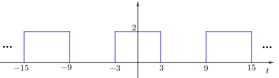
We’re going to convolve the following signals.

After taking the convolution of x and y, you'll get the following result. Remember that you can verify the results by doing the math.

- Let’s construct the signals.
First, we need a sampling frequency and a time vector so that we can create the signals on the basis of them. I’m going to use as sampling frequency Fs=200, you can use another one.
One typical and fast way to build a rectangular pulse is this
Fs=200;
Ts=1/FS; //sampling period
t= -21: Ts: 21; //time vector
x=0*t; // centered on t=0;
x(t>=-1 & t<=1)=1; //where 1 is the amplitude.
//You can use the next combination to see the results
plot(t,x);
mtlb_axis([-2 2 0 1.1]);
set(gca(),"grid",[1 1]); //grid on
Note that the function matlb_axis emulates the function of Matlab axis. Where the argument is given by [xmin xmax ymin ymax]. Therefore, you may use this function in order to handle the current axis.
After running the previous code, you will get

For the pulse train signal, we’re going to use the function squarewave(). This function generates a periodic square wave with a period of 2pi. Check its syntax
s=squarewave(t, p);
Where t is a real vector and p is the percent of the period where the signal is positive. The value is 50% by default.
Using this information we can create a pulse train as follow
//Use the same ```t``` from the previous code
y=squarewave(%pi/6*(t+3),50)+1;
clf // Clf cleans the current figure
plot(t,y);
mtlb_axis([-21 21 0 2.1]);
set(gca(),"grid",[1 1]);
Note that I’ve translated the function until get the shape I want. The result is shown in figure 12.

- Now, let’s convolve them.
If you try to use the same algorithm as in the previous section to do the convolution of two continuous-time signals, you’ll get errors. Check it out
c=conv(x,y,'same');
plot(t,c);
Then, you get this result

Note that the amplitude of the signal is wrong.
This problem is because we are using an algorithm designed for the convolution of continuous-time signals, therefore we’ll need a new one.
As you can see in figure 2, convolution between two continuous-time signals is defined as an integral. We've seen in previous tutorials that an integral can be approximated by several methods obtaining very good results. You can read it here.
We can approximate the convolution integral as follow
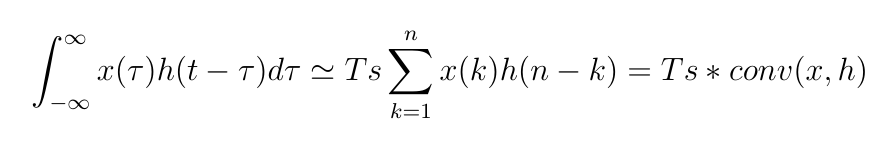
Note that this is the same as approximating the integral by adding rectangles whose widths are equal to the sampling period. Also, the expression in brackets is the formula for discrete convolution, therefore we can change our first attempt for this
c=Ts*conv(x,y,'same');
plot(t,c);
mtlb_axis([-20 20 0 4.5]);
set(gca(),"grid",[1 1]);
Take a look at the results.

Finally, we’ve got the desired result. Nevertheless, note that the amplitude shows a small error with respect to the desired value, 4. If you want to minimize the error, you can try increasing Fs.
Check the following result obtained by using Fs=1000

Observe that the error is imperceptible.
I hope you've completed this tutorial and help you to go further in Scilab and Xcos. For more tutorials take a look below.
References
- Scilab 5.5.2 Manual
- All pictures are created by me, or otherwise, they are screen captures taken from my laptop.
Curriculum
Scilab Tutorial | Approximating an integral by adding rectangular bands
Scilab Tutorial | Transformation of Control Systems Mathematical Models
Scilab Tutorial | Signal Processing: Add Echo Effect to an Audio Signal
Posted on Utopian.io - Rewarding Open Source Contributors
Hey @miguelangel2801
We're already looking forward to your next contribution!
Decentralised Rewards
Share your expertise and knowledge by rating contributions made by others on Utopian.io to help us reward the best contributions together.
Utopian Witness!
Vote for Utopian Witness! We are made of developers, system administrators, entrepreneurs, artists, content creators, thinkers. We embrace every nationality, mindset and belief.
Want to chat? Join us on Discord https://discord.me/utopian-io
Your contribution is reviewed and approved. Thank you for your contributions to open source community.
Suggestions:
Need help? Write a ticket on https://support.utopian.io.
Chat with us on Discord.
[utopian-moderator]
Thank you for your suggestions @roj