Image Reconstruction from Projections using GNU-Octave-Part 1
Introduction
One of the most amazing invention of all time is computerized tomography (CT). This invention allows to access inside a body without any damage or surgical operation. CT is a diagnostic imaging test used to create detailed images of internal organs, bones, soft tissue and blood vessels. he cross-sectional images generated during a CT scan can be reformatted in multiple planes, and can even generate three-dimensional images which can be viewed on a computer screen. for more information, please have a look at:
https://en.wikipedia.org/wiki/CT_scan
The idea behind ct scan is that when X-ray projections are passed through a body, they have different attenuation depends on the body organs. This attenuated projections are collected on the other side and then process by a method called image reconstruction to generate a cross-section of the body. Therefore, image reconstruction part plays an important role in CT scan.
What Will I Learn?
- You will learn how to generate a tomographic phantom in GNU-Octave
- You will learn How to simulate sensors around the phantom
- You will learn how to generate sensitivity maps for projections.
- Finally you will learn how to simulate Radon transform or data collection by sensors
Requirements
- Basic knowledge of tomography and image reconstruction
- GNU-Octave software downloadable from: https://www.gnu.org/software/octave/
- GNU-Octave on Github : https://github.com/NexMirror/Octave
Difficulty
- Advance
Tutorial Contents
Image reconstruction methods are used to create two-dimensional or three-dimensional images from sets of one-dimensional projections. The mathematical foundation of these reconstruction methods called Radon transform and inverse Radon transform. Collected projections are called Radon transform while the image reconstruction is called inverse radon transform.
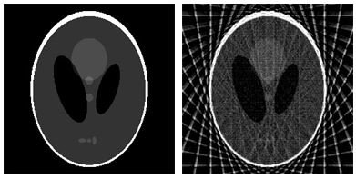
An image phantom called Shepp-Logan and its reconstructed image by inverse radon transform
There exist a lot of method to reconstruct image from projections which are divided to analytical methods include linear back projection (LBP), filter back projection (FBP), etc. and iterative methods e.g. algebraic reconstruction technique. Each of these methods have pros and cons. for example analytical methods are fast but not accurate while on the other hand iterative methods are accurate but slow. any tomography method needs three steps.
- hardware installation around a body.
- Data collection
- image reconstruction
Here we simulate the first and second steps in GNU-Octave software while we show you how to reconstruct an image from this simulation data.
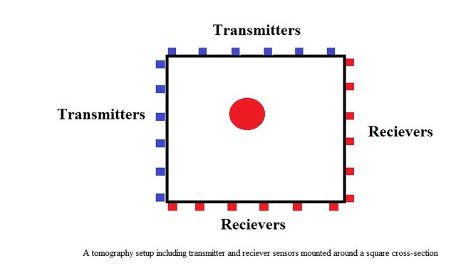
There are different setups for hardware installation. one of the simplest set up is to use only two angles as x and y to collect the data. In this way different number of sensors can be placed in two sides of a square as shown in Figure 1.
Figure 1.
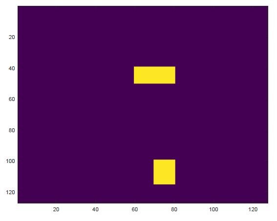
Following codes show you how to generate a phantom include two squares using GNU-Octave.
clear
clc
%% --------------- Generate a phantom -----------------------
A=zeros(127,127);
A(40:50,60:80)=1;
A(100:115,70:80)=1;
imagesc(A);*
The result is as follow:
Now is the time to simulate sensors setup around the phantom and generate projections. Here we use 10 transmitters and 10 receivers in each side of phantom following Figure 1. Therefore, total number of transmitters (receivers) are 20 for this example. For each sensor we need a sensitivity map. In tomography this step is called forward problem. These sensitivity maps are multiplied by phantom to generate the projection of the related sensor. The following codes shows the codes including sensitivity map generation.
%%  ------------- two angle sensors in x and y direction --------
N=20;  % number of sensors in each side
L=10;  % length of each sensor

%% ---------- sensitivity maps -----------------
for i=1:20
  S{1,i}=zeros(127,127);
 end
 t=1;
 for i=1:10   % Vertical projections
    b=S{1,i};
    b(1:127,t:t+9)=1;
    t=t+13;
    S{1,i}=b;
 end

  t=1;
 for i=11:20  % horizontal projections
    b=S{1,i};
    b(t:t+9,1:127)=1;
    t=t+13;
    S{1,i}=b;
    imagesc(b)
 end
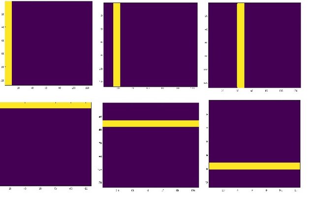
The following image shows some of the sensitivity map generated by these codes.

Now its time to multiply sensitivity maps with phantom matrix to achieve Radon space or receivers data. following codes shows how to do this step.
%% ------------ Multiplying Sensitivity map to phantom to get Radon transform or sensor data.

for i=1:20
  b=S{1,i};
  D(1,i)=sum(sum(A.*b));
  end
The output (variable D) is the Radon space (projections) data which in real world are collected by receiver sensors around the body. Here is the output for the above phantom.
D =
 Columns 1 through 18:
     0     0     0     0    33   206    54     0     0     0     0     0     0   210     0     0     0    22
 Columns 19 and 20:
   110     0
Conclusion:
In this tutorial we learn what is image reconstruction. what is a phantom and how to generate it in Octave software. what is a sensitivity map and how to generate projection using sensitivity maps. in next section we will learn about a complete data tomography setup and how to generate a Sinogram.
Curriculum
This is the first course on image reconstruction from projections.
Posted on Utopian.io - Rewarding Open Source Contributors


Your contribution cannot be approved because it does not follow the Utopian Rules.
The contribution doesn't follow the rules:
You can contact us on Discord.
[utopian-moderator]
Hi .
Sorry for this mistake.
I added Octave repository to the tutorial and posted it as a new post.
Thank you for your review.