Build Three Dimensional Plotting With Matplotlib
Introduction
Matplotlib is an open-source Python 2D plotting library which produces publication quality figures in a variety of hardcopy formats and interactive environments across platforms. Matplotlib can be used in Python scripts, the Python and IPython shell, the jupyter notebook, web application servers, and four graphical user interface toolkits.
Matplotlib tries to make easy things easy and hard things possible. You can generate plots, histograms, power spectra, bar charts, errorcharts, scatterplots, etc., with just a few lines of code.
What Will I Learn?
How to build Three Dimensional Plotting With Matplotlib ?
- You will learn three dimensional Points and Lines
- You will learn three dimensional Contour Plots
- You will learn three dimensional Wireframes and Surface Plots
- You will learn three dimensional Surface Triangulations
- You will learn Visualizing a three dimensional Möbius strip
Requirements
- Python 3.6
- Pytho Shell (Comes with Python 3.6)
- Matplotlib
Difficulty
- Basic (if you know python)
Tutorial Contents
Three Dimensional Plotting With Matplotlib
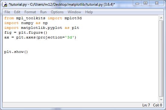
mplot3d is importing from the matplotlib library to use three-dimensional plots. We call it from the mpl toolkit for this. For that, we will use the following command:
from mpl_toolkits import mplot3d
Then, numpy and matplotlib are importing:
import numpy as np
import matplotlib.pyplot as plt
We imported the mpl toolkit. Now, we can be create three dimensional axes. We can use normal axes build command for this: projection='3d'. For that, we will use the following command:
fig = plt.figure()
ax = plt.axes(projection='3d')
Now we can display the output. For that, we will use the following command:
plt.show()
- Our commands are as followings:
- You can see the output:
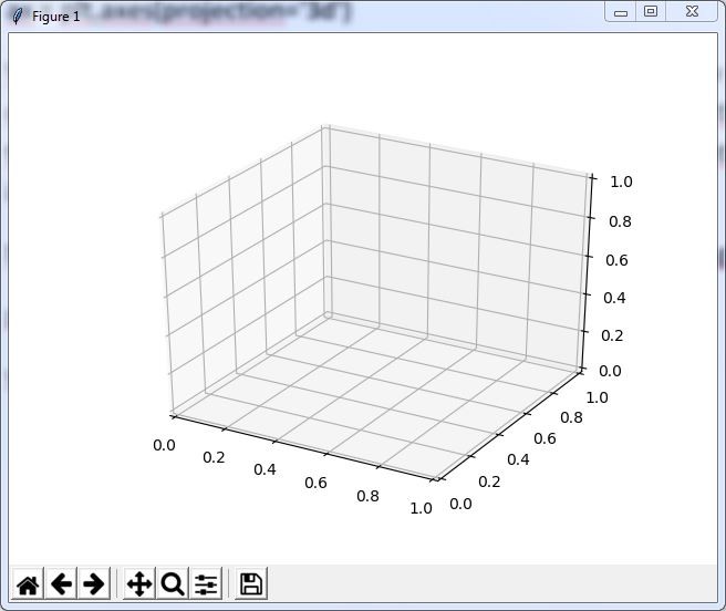
- You can see the output gif in detail below:

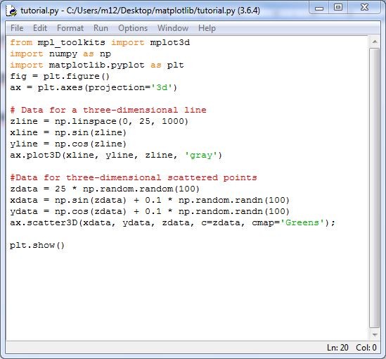
We keep going. We activated three-dimensional axes. We can build three-dimensional plot types. Let's look at 3D points and lines.
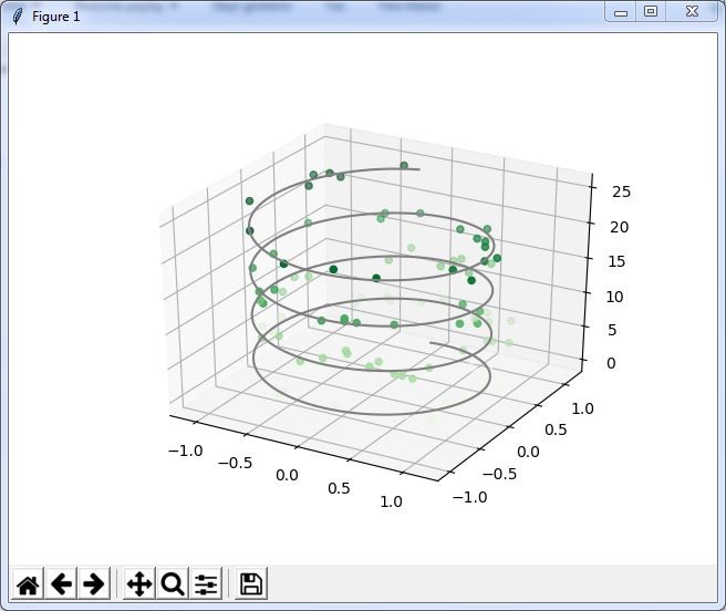
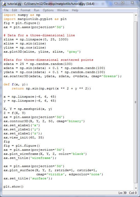
We can build three dimensional plots from sets of (x, y, z) triples. We use the ax.plot3D and ax.scatter3D commands to build them. We will plot a trigonometric spiral. This is a line along with the points.
We will start with a line. We will use # Data for a three-dimensional line for this. We will add the x, y, and z axes. We will start with the limits of the Z axis. We will use the following commands:
zline = np.linspace(0, 25, 1000)
xline = np.sin(zline)
yline = np.cos(zline)
Then, we will add color. After choosing the color, our command is as following:
ax.plot3D(xline, yline, zline, 'gray')
We will continue with points. We will use #Data for three-dimensional scattered points for this. We will add the x, y, and z Datas.
zdata = 25 * np.random.random(100)
xdata = np.sin(zdata) + 0.1 * np.random.randn(100)
ydata = np.cos(zdata) + 0.1 * np.random.randn(100)
After choosing the color, our command is as follows:
ax.scatter3D(xdata, ydata, zdata, c=zdata, cmap='Greens');
- Our commands are as following:
- Now, you can see the output:
- You can see the output gif in detail below:

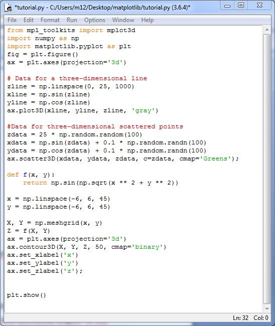
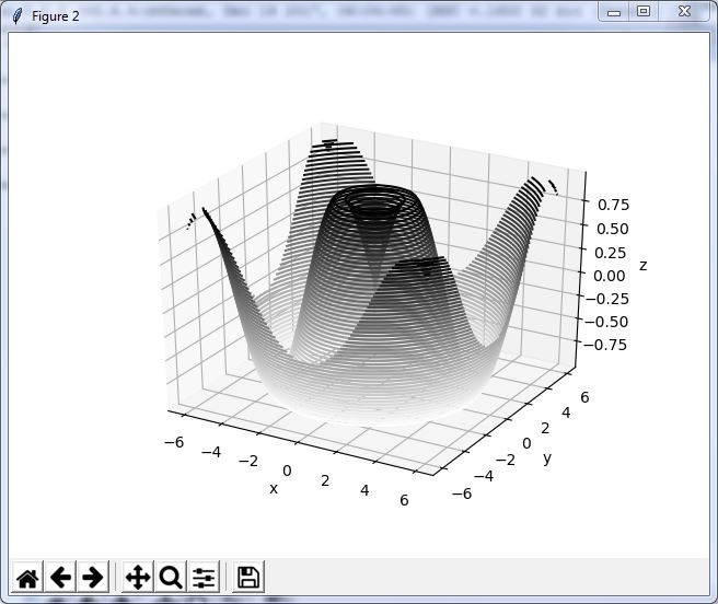
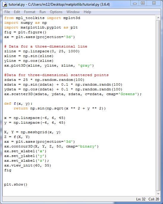
We can build three dimensional relief plots using mplot3d. The Mplot3d library offers this to us. we will build three-dimensional contour diagram of a three-dimensional sinusoidal function. It will give us a very nice structure this
` We will first use the following command for sinusoidal function:
def f(x, y):
    return np.sin(np.sqrt(x ** 2 + y ** 2))

x = np.linspace(-6, 6, 45)
y = np.linspace(-6, 6, 45)
X, Y = np.meshgrid(x, y)
Z = f(X, Y)
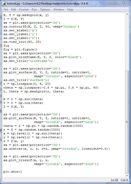
Then we will enter the build command:
fig = plt.figure()
ax = plt.axes(projection='3d')
ax.contour3D(X, Y, Z, 50, cmap='binary')
ax.set_xlabel('x')
ax.set_ylabel('y')
ax.set_zlabel('z');
- Our commands are as following:
- Now look at the output:
- You can see the output gif in detail below:

If we want, we can change the construction frequency. Let's write 150 instead of 50 and look at the output:
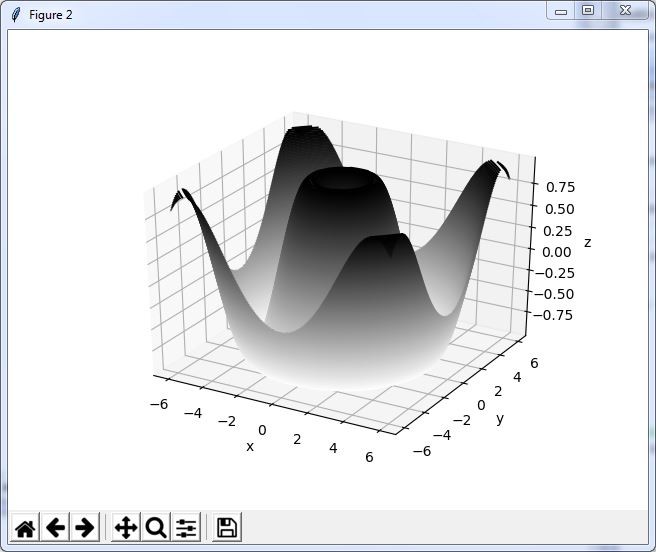
- You can see the output gif in detail below:

If the viewing angle is not appropriate we can change it. The matplotlib offers us view_int method for this. We must adjust the azimuthal angle and height to use it. We will add our command for this:
ax.view_init(60, 35)
fig
- Our commands are as following:
- Now let’s look at the output:
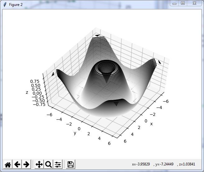
- You can see the output gif in detail below:

Now let's look at Wire Frames and Surface Plots. Also ‘mplot3D’ offers us wireframes and surface plots. They are working on gridded data. Now let's look at wireframes. We will use the following commands for this.
fig = plt.figure()
ax = plt.axes(projection='3d')
ax.plot_wireframe(X, Y, Z, color='black')
ax.set_title('wireframe');
- Our commands are as following:
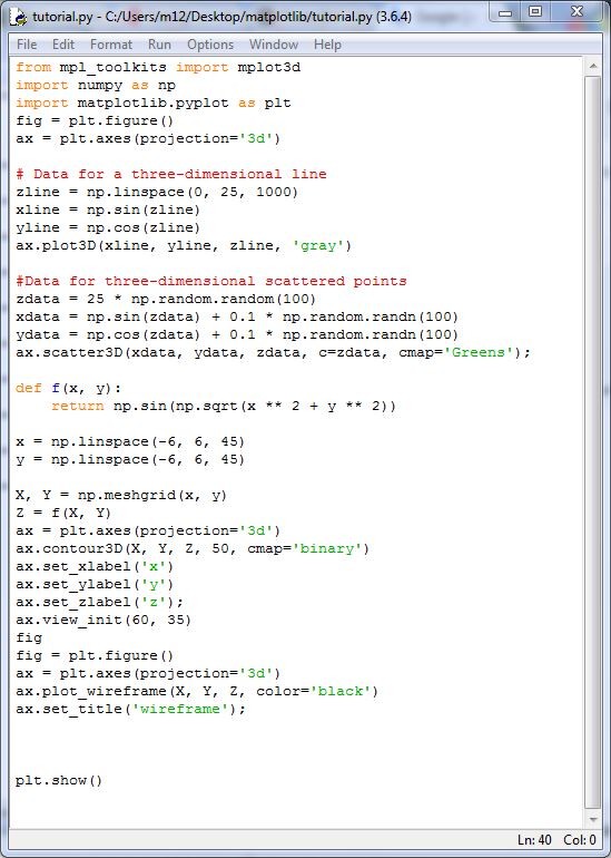
- Now let’s look at the output:
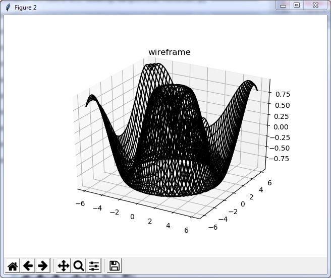
- You can see the output gif in detail below:

The surface graphics and wireframes are similar. But there is a base difference between them. The wireframe cage are filled polygons. We can make the surface clear by adding colors to the polygons. We will use the following commands for this:
ax = plt.axes(projection='3d')
ax.plot_surface(X, Y, Z, rstride=1, cstride=1,
                cmap='viridis', edgecolor='none')
ax.set_title('surface');
- Our commands are as following:
- Now let’s look at the output:
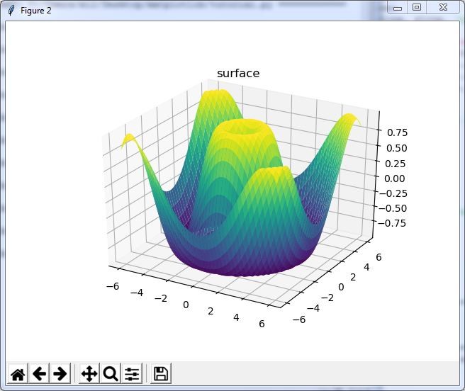
- You can see the output gif in detail below:

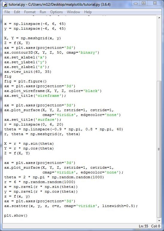
We can give this plots a slice. We will use the following commands for this:
r = np.linspace(0, 6, 20)
theta = np.linspace(-0.9 * np.pi, 0.8 * np.pi, 40)
r, theta = np.meshgrid(r, theta)

X = r * np.sin(theta)
Y = r * np.cos(theta)
Z = f(X, Y)

ax = plt.axes(projection='3d')
ax.plot_surface(X, Y, Z, rstride=1, cstride=1,
                cmap='viridis', edgecolor='none');
Also, matplotlib offers Surface Triangulations us. We can create a scatter plot of the points. This will give us an idea about the surface. We will use the following commands for this:
theta = 2 * np.pi * np.random.random(1000)
r = 6 * np.random.random(1000)
x = np.ravel(r * np.sin(theta))
y = np.ravel(r * np.cos(theta))
z = f(x, y)
ax = plt.axes(projection='3d')
ax.scatter(x, y, z, c=z, cmap='viridis', linewidth=0.5);
- Our commands are as following:
- Now let’s look at the output:
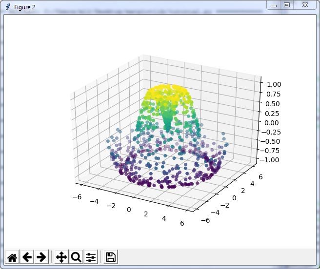
- You can see the output gif in detail below:

We can create a set of triangles between adjacent points. The command that build it: ax.plot_trisurf. We will use the following commands for this:
ax = plt.axes(projection='3d')
ax.plot_trisurf(x, y, z,
                cmap='viridis', edgecolor='none');
- Our commands are as following:
- Now let’s look at the output:
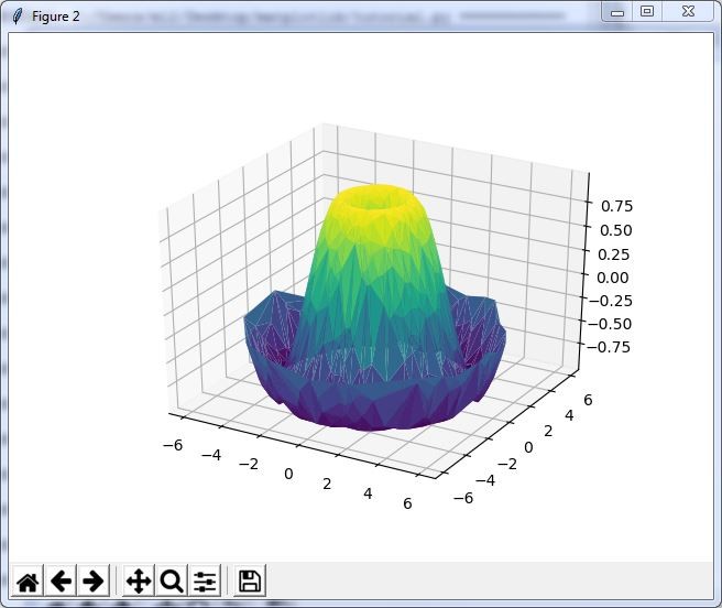
- You can see the output gif in detail below:

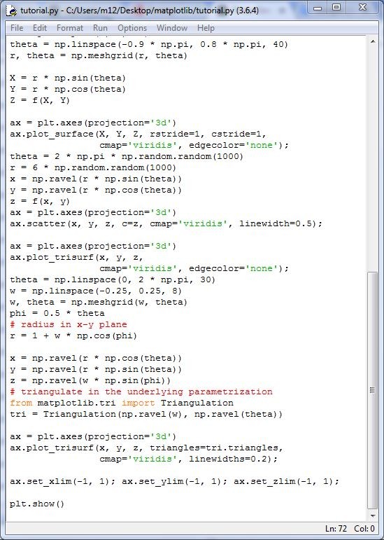
Also, it is possible to plot a three-dimensional Möbius strip using matplotlib. Let's see how we build möbius strip. We will visualize the Möbius strip object using Matplotlib's three-dimensional tools. We will use the following commands for this:
theta = np.linspace(0, 2 * np.pi, 30)
w = np.linspace(-0.25, 0.25, 8)
w, theta = np.meshgrid(w, theta)
Now let's continue building möbius strip. We will use the following commands for this:
phi = 0.5 * theta
We can use recollection of trigonometry to derive the three-dimensional embedding. We will use the following commands for this:
# radius in x-y plane
r = 1 + w * np.cos(phi)

x = np.ravel(r * np.cos(theta))
y = np.ravel(r * np.sin(theta))
z = np.ravel(w * np.sin(phi))
We must make sure that the triangulation process is correct at the end. This can be accomplished as follows. We will use the following commands for this:
# triangulate in the underlying parametrization
from matplotlib.tri import Triangulation
tri = Triangulation(np.ravel(w), np.ravel(theta))

ax = plt.axes(projection='3d')
ax.plot_trisurf(x, y, z, triangles=tri.triangles,
                cmap='viridis', linewidths=0.2);

ax.set_xlim(-1, 1); ax.set_ylim(-1, 1); ax.set_zlim(-1, 1);
- Our commands are as following:
- Now let’s look at the output:
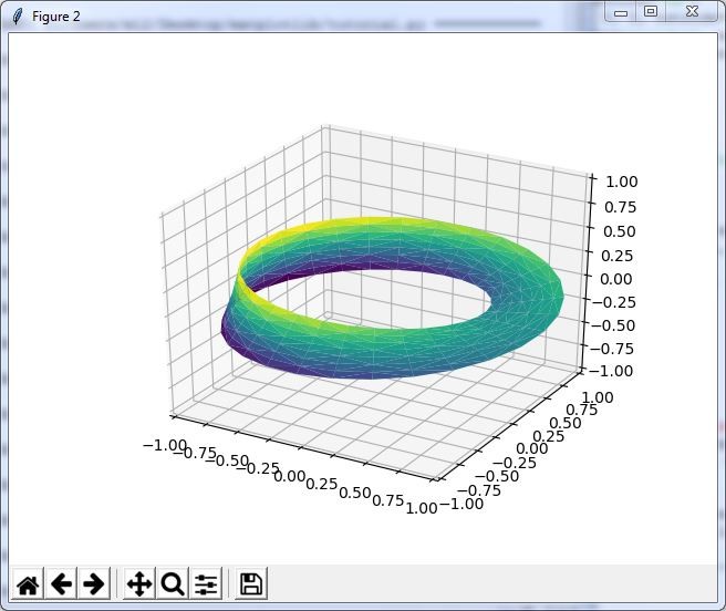
- You can see the output gif in detail below:

Today, we built three dimensional plotting using Matplotlib with the help of python shell at the first study. We learned the build codes of very useful structures. Thank you for studying the course.
Source
Posted on Utopian.io - Rewarding Open Source Contributors
@emirfirlar, No matter approved or not, I upvote and support you.
Thank you for supporting me @steemitstats
Your contribution cannot be approved because it is a plagiarism.
Source
You can contact us on Discord.
[utopian-moderator]
Thanks for informing. My purpose was not plagiarism. I prepared the content by changing
the codes as possible. I prepared the content myself. Also, i have already specified it as source at 4. But refusing is your decision and I respect it.
Congratulations! This post has been upvoted from the communal account, @minnowsupport, by emirfirlar from the Minnow Support Project. It's a witness project run by aggroed, ausbitbank, teamsteem, theprophet0, someguy123, neoxian, followbtcnews, and netuoso. The goal is to help Steemit grow by supporting Minnows. Please find us at the Peace, Abundance, and Liberty Network (PALnet) Discord Channel. It's a completely public and open space to all members of the Steemit community who voluntarily choose to be there.
If you would like to delegate to the Minnow Support Project you can do so by clicking on the following links: 50SP, 100SP, 250SP, 500SP, 1000SP, 5000SP.
Be sure to leave at least 50SP undelegated on your account.
This post has received a 0.24 % upvote from @drotto thanks to: @banjo.