[Custom Thumbnail]
All the Code of the series can be found at the Github repository: https://github.com/drifter1/circuitsim

---

Introduction

    Hello it's a me again @drifter1! Today we continue with the Electronic Circuit Simulation series, a tutorial series where we will be implementing a full-on electronic circuit simulator (like SPICE) studying the whole concept and mainly physics behind it! In this article we continue with the Implementation of a complete simulator for Static Analysis. In this third and final step we will loop through the components list of the last article(s) to fill the MNA Matrices and solve the MNA System...

Requirements:

• Physics and more specifically Electromagnetism Knowledge
• Knowing how to solve Linear Systems using Linear Algebra
• Some understanding of the Programming Language Python

Difficulty:

Talking about the series in general this series can be rated:

• Intermediate to Advanced

Today's topic(s) can be rated:

• Intermediate

---

Actual Tutorial Content

Fill MNA Matrices

    In the Modified Nodal Analysis (MNA) articles I talked you through the whole mathematics that give us the linear system, which solves Electronic Circuits for Node potentials and currents through Group 2 components. The final linear system that we got for Static Analysis is:


As we showed in this article, the A-matrix contains 4 matrices:

• G → Conductance matrix:
• each line and row corresponds to a specific node
• diagonal is positive and containing the total "self" conductance of each node
• the non-diagonal are negative and containing the mutual conductance between nodes
• B → Group 2 component incidence matrix:
• each column corresponds to a specific Group 2 component (voltage source)
• '1' when node connected to '+' pole, '-1' when node connected to '-' pole and '0' when not incident
• C → Transpose of B
• D → All-zero when only independent sources are considered

    The b-matrix on the other hand contains the constant output of all independent sources (current and voltage), with the current values following the logic:

• positive when entering the node
• negative when leaving the node

FIlling Procedure

In our Code we will have to:

1. Calculate the number of Group 2 components and the Matrix size
2. Define the matrices as numpy arrays (A is two-dimensional, b is one-dimensional)
3. Define a variable that keeps track of the current Group 2 component index to help us fill the correct spot in the Matrices
4. Loop through all the components and fill the Matrices depending on their type:
• Resistance affect the G-matrix of A
• Capacitance is an open circuit in Static Analysis
• Inductance works like an closed circuit with 0 resistance and 0 voltage affecting the B and C matrices of A and the b-matrix with a value of '0'
• Voltage sources affect the B and C matrices of A and the b-matrix with their value
• Current sources only affect the b-matrix with negative impact on the high node and negative impact on the low node

Python Code

The Code looks like this:

def calculateMatrices(components, nodeCount):

    # use global scope variables for component counts
    global voltageCount, inductorCount

    # calculate g2 components
    g2Count = voltageCount + inductorCount
    print("Group 2 count:", g2Count)

    # calculate matrix size
    matrixSize = nodeCount + g2Count - 1
    print("Matrix size:", matrixSize, "\n")

    # define Matrices
    A = np.zeros((matrixSize, matrixSize))
    b = np.zeros(matrixSize)

    # Group 2 component index
    g2Index = matrixSize - g2Count

    # loop through all components
    for component in components:
        # store component info in temporary variable
        high = component.high
        low = component.low
        value = component.value

        if component.comp_type == 'R':
            # affects G-matrix of A
            # diagonal self-conductance of node
            if high != 0:
                A[high - 1][high - 1] = A[high - 1][high - 1] + 1/value
            if low != 0:
                A[low - 1][low - 1] = A[low - 1][low - 1] + 1/value

            # mutual conductance between nodes
            if high != 0 and low != 0:
                A[high - 1][low - 1] = A[high - 1][low - 1] - 1/value
                A[low - 1][high - 1] = A[low - 1][high - 1] - 1/value

        # elif component.comp_type == 'C':
            # Capacitance is an open circuit for Static Analysis

        elif component.comp_type == 'L':
            # closed circuit  in Static Analysis: 0 resistance and 0 voltage
            # affects the B and C matrices of A
            if high != 0:
                A[high - 1][g2Index] = A[high - 1][g2Index] + 1
                A[g2Index][high - 1] = A[g2Index][high - 1] + 1
            if low != 0:
                A[low - 1][g2Index] = A[low - 1][g2Index] - 1
                A[g2Index][low - 1] = A[g2Index][low - 1] - 1

            # affects b-matrix
            b[g2Index] = 0

            # increase G2 index
            g2Index = g2Index + 1

        elif component.comp_type == 'V':
            # affects the B and C matrices of A
            if high != 0:
                A[high - 1][g2Index] = A[high - 1][g2Index] + 1
                A[g2Index][high - 1] = A[g2Index][high - 1] + 1
            if low != 0:
                A[low - 1][g2Index] = A[low - 1][g2Index] - 1
                A[g2Index][low - 1] = A[g2Index][low - 1] - 1

            # affects b-matrix
            b[g2Index] = value

            # increase G2 counter
            g2Index = g2Index + 1

        elif component.comp_type == 'I':
            # affects b-matrix
            if high != 0:
                b[high - 1] = b[high - 1] - value
            if low != 0:
                b[low - 1] = b[low - 1] + value

    return A, b

Don't forget to import the numpy library using:

import numpy as np

---

Solve MNA System

    To solve the MNA System we basically only have to call the "np.linalg.solve()" function. So, the Code for solving is:

def solveSystem(A, b):
    x = np.linalg.solve(A, b)
    return x

Let's tweak the main function from last time...

# Initialize component counters
voltageCount = 0
currentCount = 0
resistorCount = 0
capacitorCount = 0
inductorCount = 0

# Parse File
fileName = "example.spice"
print("Parsing file...\n")
components = parseFile(fileName)

# Map nodes
print("Mapping nodes...\n")
components, hashtable = mapNodes(components)

# Print Information
print("Circuit Info")
print("Component count: ", len(components))
print("Voltage count: ", voltageCount)
print("Current count: ", currentCount)
print("Resistance count: ", resistorCount)
print("Capacitance count: ", capacitorCount)
print("Inductance count: ", inductorCount)
print("Node count: ", hashtable.nodeCount)

print("\nNodes are mapped as following:")
for key, val in hashtable.nodes.items():
    print("\"" + key + "\" :", val)

print("\nCircuit Components:")
for i in range(0, len(components)):
    print(components[i])

# Calculate and solve system
print("\nCalculating MNA Matrices...\n")
A, b = calculateMatrices(components, hashtable.nodeCount)
print("A:\n", A)
print("b:\n", b)

print("\nSolving System...\n")
x = solveSystem(A, b)
print("x:\n", x)

    The numpy arrays are printed out with maximum precision and scientific notation. To get rid of it and make them print out in a more"pretty" way, let's define the following print options:

np.set_printoptions(precision=3, suppress=True)

---

Running the Examples

Simple Example

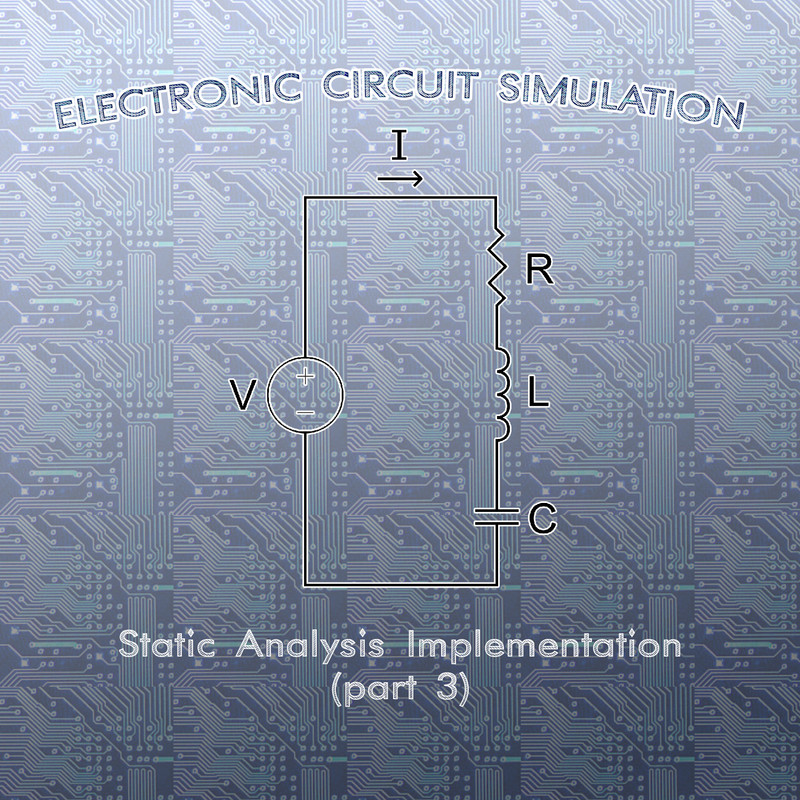
Suppose the simple circuit (that we used way to often):


Running our simulator for this simple example we get:


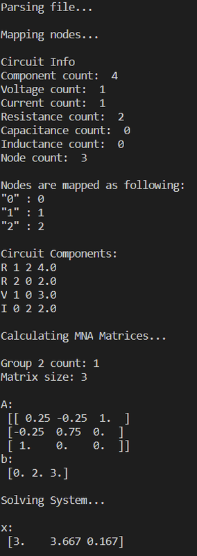
    You can see that the system got filled with the same values that we found in the article Modified Nodal Analysis (part 2), which was:


    Of course it also gives us the same solution that we got with "manual" Code! Having the same exact order in the solution was just random luck, as the nodes could have been mapped way differently giving us a mixed up solution! That's exactly what happens in more advanced circuits...

Advanced Circuit 1

Running our simulator for the first Netlist of the previous article we get: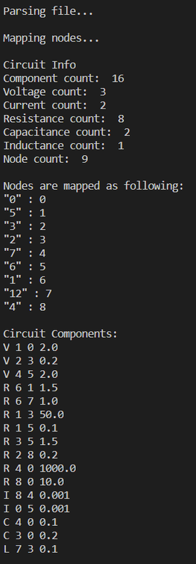

Advanced Circuit 2

Running our simulator for the second Netlist of the previous article we get:



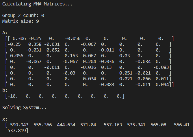
The last two circuits would take much more time to solve "by hand"!

    And with that we are actually finished with the Implementation for Static Analysis, or are we? Well, the A matrix contains lots of zeros and so we are not really that memory optimized right now. To optimize our simulator we can use a so called Sparse matrix to store the two-dimensional array A, which is exactly what we will be doing next time!

---

RESOURCES

References:

1. https://www.geeksforgeeks.org/python-numpy/

Mathematical Equations were made using quicklatex

---

Previous parts of the series

Introduction and Electromagnetism Background

• Introduction
• Electromagnetism Background (part 1)
• Electromagnetism Background (part 2)

Mesh and Nodal Analysis

• Mesh Analysis
• Nodal Analysis
• Modified Mesh Analysis by Inspection
• Modified Nodal Analysis by Inspection

Modified Nodal Analysis

• Incidence Matrix and Modified Kirchhoff Laws
• Modified Nodal Analysis (part 1)
• Modified Nodal Analysis (part 2)

Static Analysis

• Static Analysis Implementation (part 1)
• Static Analysis Implementation (part 2)

---

Final words | Next up on the project

    And this is actually it for today's post and I hope that you enjoyed it!

    Next time we will talk about Sparse Matrices, which will be used to optimize our Simulator for Memory, as we will not store 0 values anymore...

So, see ya next time!

---

GitHub Account:

https://github.com/drifter1

Keep on drifting! ;)