Obtaining the Transfer Tunction G(s) of a Control System Using the Mason Formula | Example 1

reyito (45)in #steemtem • 6 years ago (edited)

Hello friends of Steemit, nice to say hello!

In this document I will show you through an exercise how to obtain the transfer function G (S) of a linear control system using the Mason formula. The aforementioned formula is very useful in the study of control systems whatever the discipline (electrical, electronic, mechanical, systems, among others) or the nature of the problem to be addressed. The exercise developed in this article was taken from one of my classes taught to engineering students, specifically in the subject "SYSTEMS". It is based on a linear control system with an input signal and an output signal (SISO: "Single Input / Single Output"). We will start the theme with the simple definition of what a transfer function is, we will see the concept of what a "block diagram" is, and what a "signal flow diagram" consists of, to finally present the Mason formula and its application I hope that this exhibition will be very useful for those who are familiar with the aforementioned topic, and for those who have not had the opportunity to interact with this wonderful and fascinating field of knowledge, I invite you to try to understand the content. Welcome everyone.

Ogata (1989) argues that in the field of systems theory, the transfer functions "(...) are frequently used to characterize the input and output relationships of systems of linear differential equations, invariant in time (...) and is defined as the relation of the Laplace transform of the output (response function) and the Laplace transform of the input (drive or excitation function) under the assumption that all the initial conditions are zero "(p.389 ).

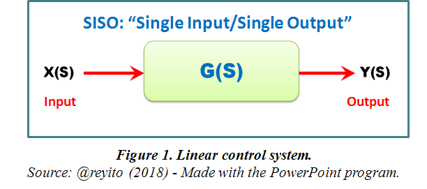
According to the above, the transfer function G(s) of a control system is a mathematical expression that allows knowing the relationship between the input signal X(s) and the output signal Y(s), as shows in Figure 1.

Thus:

Where: X(s), Y(s) and G(s) correspond to the Laplace transforms of the functions in the time domain x (t), and (t) and g (t), respectively. It is important to note again that the calculation of a transfer function (FDT) assumes that the initial conditions are equal to zero. On the other hand, it is worth remembering that the variable "S" belongs to the field of complex numbers; in this case s = jω, where $j=\sqrt{-1}$ (imaginary unit) and $\omega =2\pi f$ (angular frequency in rad / s with f = oscillatory frequency in Hz). In general, the complex variable "s" is given by $s=\sigma +j\omega$ , but for the calculation of the FDT, the attenuation factor (σ = 0) is considered zero. Given that the scope of this document is merely to present the Mason formula (FDM), it is irrelevant to delve into the reasons that lead to consider the effect of attenuation of the signals as null, which is left to the discretion of the reader and his / her restlessness of wanting to delve into the subject.

Types of input signals commonly used:

Impulse signal (Dirac Delta): $\delta \left ( t \right )$
Single step signal: $u\left ( t \right )$
Unitary ramp signal: $r\left ( t \right )$
Sinusoidal signal: $sen\left ( t \right )$

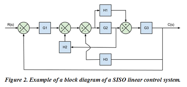
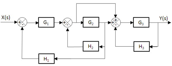
According to Ogata (1998), a block diagram of a system "is a graphic representation of the functions performed by each component and the flow of the signals (...) and describes the interrelationships that exist between the different components. The transfer functions of the components usually get into the corresponding blocks "(p.497). In other words, a block diagram contains arrows that indicate the direction in which the signals that intervene in the system flow (input signals, output signals, internal signals, disturbances), and rectangles (blocks) which represent the parts of a system or process (plant, controllers, actuators, feedback, among others) conceived as a "black box" in which the intrinsic characteristics that give rise to the transfer functions (gains) of each block are present; in one way or another they will influence the overall behavior of the original system. When the internal parameters of the blocks are constant, differential equations are generated with coefficients that are also constant which means that the system is invariant in time, in other words, the internal properties of the system remain intact in the face of time; otherwise we would be talking about a variant system over time; we will deal with the first of the cases. Figure 2 shows an example of a block diagram.

Source

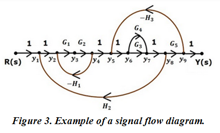
In Figure 2, the H correspond to the gains of the feedback loops, while the G correspond to the gains of the direct loops. The circles represent SUMATERS, which receive or admit various input signals and generate an output that is the algebraic sum of their corresponding inputs.

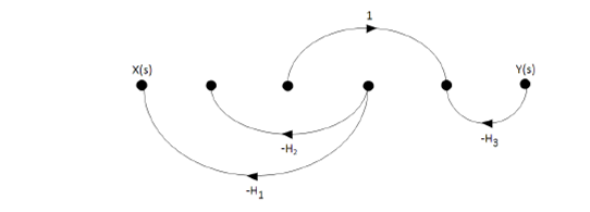
The signal flow diagram (SFD) is obtained from the block diagram; that is, it can be seen as a simplified version of a block diagram. An example is shown in Figure 3.

Sourse

Properties of the signal flow diagrams:

The most commons are:

Simplification of Series Earnings.
Simplification of Profits in Parallel.
Elimination of Internal Nodes.
Elimination of ties.

The total gain G(s) of a signal flow diagram, between the input node and the output node and containing several direct paths, is determined by the following equation:

Developing the summation, it results:

Where:

∆ : Determinant of the signal flow diagram (complete graph) and determined by the formula:

X (s): Input variable (represents the input signal).
Y (s): Output variable (represents the output signal).
G (s): Gain of the complete system between Y (s) and X (s).
n: Number of possible paths (paths) possible between Y (S) and X (S).
$G_{k}$ : Gain on the kth path from the input node to the output node and which is equal to the product of the gains of the branches that make up the trajectory.
$L_{i}$ : Gain of all simple ties.
$L_{i}L_{j}$ : Product of the profits of the disjoint ties taken two by two.
$L_{i}L_{j}L_{k}$ : Product of the profits of disjoint ties taken from three in three.
$\Delta _{k}$ : He is the cofactor of $G_{k}$ , that is, the determinant of the sub-graph that remains when the trajectory is removed (removed) $G_{k}$ . (Note: $\Delta _{k}$ is defined in the same way as the determinant Δ of the signal flow diagram, only that the substituted gains in the formulas correspond to the loops that do not touch the direct k-th path).

Obtain the transfer function G (s) of a control system whose block diagram is shown in the following figure, applying the Mason formula.

SOLUTION

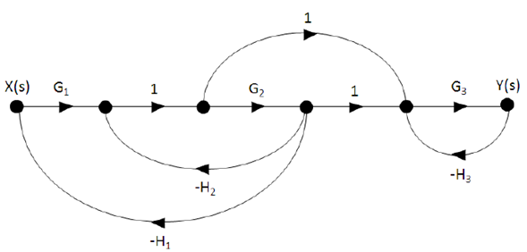
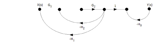
Step # 1: Construction of the signal flow diagram.

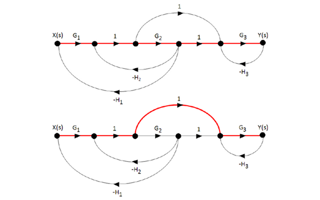
Step # 2: Identification of direct roads.

There are two direct paths (n = 2) identified with the red color in the following diagram.

Mason's formula for n = 2:

$\left ( I \right )\: \: \: \: \: G\left ( S \right )=\frac{1}{\Delta }\sum_{k=1}^{2}G_{k}\Delta _{k}=\frac{G_{1}\Delta _{1}+G_{2}\Delta _{2}}{\Delta }$

According to (I) we must find the gains of the direct paths ( $G_{1}$ y $G_{2}$ ), the determinant (Δ) and the cofactors ( $\Delta _{1}$ y $\Delta _{2}$ ) .

Step # 3: Determination of the gains of the direct roads.

For k=1: 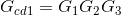$G _{cd1}=G _{1}G _{2}G _{3}$ (II)
For k=2: $G _{cd2}=G _{1}G _{3}$ (III)

Step # 4: Identification of all loops or loops in the system.

$L _{1}=-G _{1}G _{2}H _{1}$ (IV)
$L _{2}=-G _{2}H _{2}$ (V)
$L _{3}=-G _{3}H _{3}$ (VI)

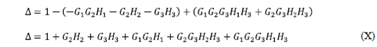
Step # 5: Determination of the determinant Δ.

We know that:

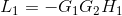
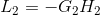
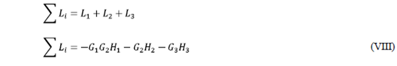
Sum of all the profits of the ties:

Sum of the profits of disjoint ties taken from two in two:
The following is observed in the signal flow diagram:

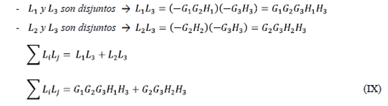
Sum of the profits of disjoint ties taken from three in three:
In the DFS it is observed that they DO NOT EXIST!

We substitute (VIII) and (IX) in (VII):

Step # 6: Determining the cofactor $\Delta _{1}$

We must remove (remove) from the signal flow diagram the direct path $G _{cd1}$ , and the same graph is applied to the resulting graph for the calculation of Δ (see the following figure).

Sum of all the profits of the ties:
There are no ties, therefore the result is ZERO.
Sum of the profits of disjoint ties taken from two in two:
There are no disjoint ties, therefore the result is ZERO.

Step # 7: Determination of the cofactor $\Delta _{2}$

We must remove (remove) from the signal flow diagram the direct path $G _{cd2}$ , and the same graph is applied to the resulting graph for the calculation of Δ (see the following figure).

Sum of all the profits of the ties:
There are no ties, therefore the result is ZERO.
Sum of the profits of disjoint ties taken from two in two:
There are no disjoint ties, therefore the result is ZERO.

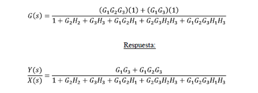
Step # 8: Determination of the transfer function of the control system.
We substitute (II), (III), (X), (XI) and (XII) into (I).

CONCLUSIONS

Despite the fact that the method results, IN APPEARANCE, somewhat cumbersome, paradoxically it is relatively easy to understand and apply, and I consider it appropriate to conclude by answering a very important question:

The answer is very simple: We do it because, in general, most of the real control systems present a high level of complexity given the number of interconnection loops and feedback loops that make it up, which makes it very difficult to obtain G (s) by the methods of mathematical simplification that we commonly know, the risk of making mistakes is tendentiously greater. On the other hand, the probability of making mistakes is much lower when applying the Mason formula because we save the intermediate steps of the traditional method.

Once the transfer function is known, it can be used to carry out further studies related to the STABILITY of the control system based on the location of the poles in the complex plane, which are obtained from the characteristic polynomial.

You can verify the ways in which both the magnitude and the angle of the transfer function vary with the frequency (Bode diagrams), and thus specify the range or range of frequencies for which a certain behavior in the graphic response is observed of the system.

BIBLIOGRAPHY

#steemstem #knowledge #engineering #technology

6 years ago in #steemtem by reyito (45)

$0.00

STEEM 0.30

TRX 0.12

JST 0.032

BTC 58557.01

ETH 2992.97

USDT 1.00

SBD 3.74