Towards Artificial Minds 2: The Basics of Artificial Intelligence

Basics of Artificial Intelligence

As written above, research on artificial intelligence is going on since over 60 years. During this time a lot of different approaches for creating intelligent systems were developed, another reason for the manifold approaches to artificial intelligence is that the phenomenon of intelligence isn't really a crisply defined concept. Thus, when writing about the basics of artificial intelligence, I can only briefly introduce some of these concepts¹. One thing that all approaches of artificial intelligence have in common is, that they can be defined with a mathematical notation and that they rely on computation, so that they can be executed on a computing device.

The dominating paradigm during the early days of artificial intelligence was called symbolic artificial intelligence, problem solving by searching, first-order logical inference and knowledge representation using logic were some approaches back in the day. Even though they still do have some eligibility today, nowadays these approaches are known as "Good Old-Fashioned Artificial Intelligence" (GOFAI), a term first used by John Haugeland in 1985 [Hau85]. AI researchers, as well as cognitive scientists, came to the conclusion, that the world is too complex for a pure symbol processing approach.

In order to solve this problem, the focus has shifted from symbolic processing to probabilistic models and statistical learning². Instead of doing processing on abstract symbols, statistical inferences are now used to make systems "intelligent". A lot of research on statistics has been incorporated into artificial intelligence. A special kind of statistical "knowledge" representation, which is very commonly used in artificial intelligence are neural networks.

Probabilistic and statistical models have the big advantage that they are able to handle the complexity of the world in a much better way than GOFAI approaches do, but they need a lot of input data to extract the relevant features and it is in general not apparent from a model, why it works the way it does, neural networks for example are black boxes where the concrete internal processes that are responsible for an output are not transparent.

Interpolation

Linear Regression

Figure 1: Example for linear regression. The blue dots are the data samples, the red line is the interpolated relationship between all the data samples.

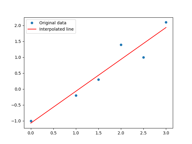
Linear regression is a statistical approach to model the relationship between a depended variable and a one or more independent variables. It interpolates a line through all data samples that resembles a linear relationship between the different dimensions of the samples³. The offset and the steepness of this line are dependent on the distribution of the input data: it tries to minimise the distance of every data sample and the interpolated line. See figure 1 for a graphical representation of linear regression. The interpolation is represented through the following equation:

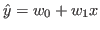  (1)

The parameter w₀ is the offset of the line, the parameter w₁ is the steepness of the line and x is the x-value for which we want to interpolate the y-value. Both w₀ and w₁ are also called weights. In order to find the interpolation line that has the shortest distance to every data sample, we need to minimise the error of the prediction ŷ and the actual value y. This can be done by computing the mean squared error (MSE) and adjusting the weights w₀ and w₁ accordingly:

  (2)

N is the number of data samples, so we have to minimise the mean squared error for all data samples. In order to adjust the weights, we just have to compute the derivative of the MSE, set the result zero and solve the equations with respect to the weights:

  (3)
  (4)

Polynomial Curve Fitting

Figure 2: Polynomial curve fitting for polynomials of a different order M. If M = 0 the "curve" is just a flat line, that can only be moved vertically, depending on the sample data (so that the distance to all points of the sample data is minimised). If M = 1 the "curve" is still just a line, but it is not flat and its steepness and direction of its slope depend also depend on the sampled data points. Note that this special case of (polynomial) curve fitting is equivalent to linear regression. In this example M = 3 is the best interpolation: the fitted curve (in red) roughly approximates the original function. If too many polynomials are chosen (in this case M = 9), the interpolated curve is "overfitting", meaning that the model to interpolate the curve is contains too many parameters to be justified by the data samples and so the interpolation is osculating between the points instead of following their real distribution. This figure was taken from [Bis06]

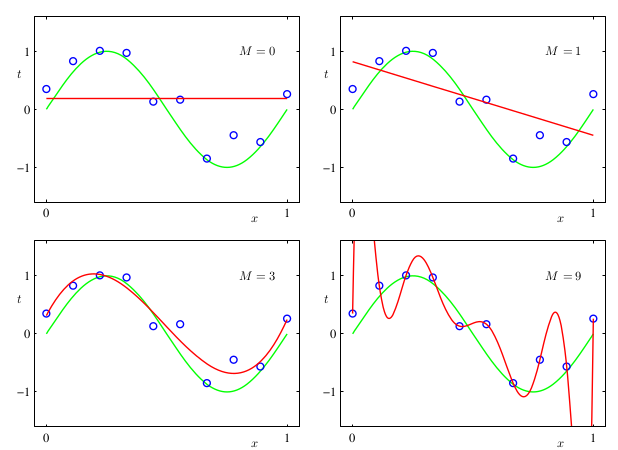
Curve fitting is related to linear regression, while linear regression tries to find a linear relationship between statistical variables, curve fitting tries to interpolate a function for given points. Both are using more or less the same technique⁴. Figure 2 shows the relation between linear regression and polynomial curve fitting.

Polynomial curve fitting is also done by minimising the mean squared error (c.f. equation 2), the resulting equations to minimise are similar to equation 3 and equation 4, but slightly more complex, depending on which polynomial is chosen.

What we can see here is, that "training" a statistical model is basically an optimisation problem: the values of the different weights w has to be selected in such a way, that they are optimal. Linear regression and polynomial curve fitting have the feature that an analytical solution exists, the approach I described above guarantees that the weights are optimal for the given data samples. I admit, that at first all of this doesn't look very impressive, it is just high-school maths. But the interesting thing about this high-school maths is, that it is the very foundation for the most advanced artificial intelligence systems that we know today. Neural networks (which I'm going to introduce in more detail in the next subsection) follow the same basic principle of trying to fit a function to given data samples. Although I also have to admit, that things can (and will) get much more complex than this and easements like the existence of an analytical solution do not exist any more. "Fitting a curve" can be seen as the very foundation for artificial intelligence today, note that GOFAI does not really deal with function approximation, but with different problems (which can also be translated into a "curve fitting" problem). Even though the problems are of statistical nature, the approaches to solving them is not only statistical, but it combines approaches from linear algebra and calculus as well.

Neural Network

Artificial neural networks are computing systems that are inspired by the information processing capabilities of human and animal brains⁵. They are universal function approximators [Csá01], meaning that they are able to approximate any continuous function. As stated in the previous subsection, artificial intelligence is very concerned with approximating functions⁶. The idea of neural networks is actually a very old one and dates back to 1960 [WH60], during the last five decades the idea of artificial neural networks used to fall out of favour several times, but always managed to get back in fashion again. The reason for this are the overwhelming computational demands involved in training such a neural network, which kept them from being practical, while other approaches at the time delivered better results and demanded less computational resources. Since roughly ten years neural networks are again back in fashion, due to advances made in deep learning [Hin07] and are basically responsible for every major breakthrough in artificial intelligence made in the last decade.

Figure 3: Schematic layout of an artificial neural network. This neural network consists of one input layer x, one hidden layer z and one output layer y, this neural network is a feed-forward network, which means that the inputs get propagated forward in order to produce an output. Every neuron of the input layer is connected with every neuron of the hidden layer and every neuron of the hidden layer is connected with every neuron on the output layer. A neural network can have more than just one hidden layer, this allows the network to learn a more abstract representation, but is also computationally more expensive. Figure take from [Bis06].

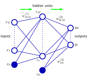
Similar to linear regression and polynomial curve fitting, the learning happens by adjusting the weights w to fit the input samples. A neural network consists of neurons that are connected with other neurons from the next layer, each neuron has an activation function, when the activation threshold is reached, the neuron "fires", the weight w from the firing neuron is then multiplied with the output of that neuron and used as input for the neurons in the next layer. A neuron in the next layer sums up all the inputs it receives and if those inputs are larger than the threshold value it fires again and is used as input for the neurons in the following layer.

For example the neuron z₁ from hidden layer of figure 3 receives the following input:

  (5)

Where D is the number of input neurons x and σ is the activation function that decides whether a neuron fires or not. An activation function can be any function, but for in order to be able to train the network using the backpropagation algorithm (more about that soon), it has to be a continuous function, so it is differentiable. A commonly used activation function is the sigmoid function:

  (6)

Training a neural network (adjusting the weights so that the error function is minimised) used to a big problem for neural networks and led to them falling out of favour, in 1974 the first version of the backpropagation algorithm was introduced [Wer74], which solved the credit assignment problem (how much is one single weight involved in the error) and allowed to train neural networks in a more efficient way. Unlike linear regression and polynomial curve fitting, neural networks can not be optimised in an analytical way, which means that the weights of a neural network have to be updated in an iterative process. Also, unlike linear regression, the space in which we are looking for the optimal weights of a neural network is high dimensional, which adds additional complexity to the optimisation process. Backpropagation is "going down" the steepest gradient in order to find a minimum. Since there can be more than one minimum it is possible to get stuck in a local minimum and thus only finding a suboptimal solution instead of finding the optimal global minimum. To avoid this there are several techniques that can be applied.

With neural networks overfitting is also possible, this happens, when the neural networks are too well-adjusted to the training data and are not able to generalise for previously unseen data samples, the network learned the features of the train samples "by heart".

There are a lot of different types of artificial neural networks and motivated from the recent breakthroughs there is a lot of research is going on in this domain right now, mostly in artificial intelligence, but also in related fields like cognitive science, where neural networks are a key component in the connectionist paradigm.

Reinforcement Learning

So far I only wrote about finding the underlying distribution for a given data samples in order to make predictions for previously unknown data samples. In artificial intelligence/machine learning this is called supervised learning, since each data sample has an input and a target value. Because those methods have a target value, training them is basically "to fit a curve", as mentioned above. But this comes with a drawback: we need labelled data, all input data needs to have target values. Creating labelled input data is a very expensive task and in some cases just not feasible. In order to tackle this problem different techniques have been developed: unsupervised learning and reinforcement learning. Unsupervised learning is about finding similarities and clusters in unlabelled data, reinforcement learning is about reinforcing actions that help to reach a set goal. In this subsection I am going to elaborate this a bit more.

Just like artificial neural networks, reinforcement learning is inspired by findings in neuroscience: human and animal brains have mechanisms that reinforce "good" behaviour⁷, meaning that certain actions cause the brain to give itself a reward. Kenji Doya wrote a very good introduction to reinforcement learning and connected it with the neural mechanisms that are happening in biological brains [Doy02].

One big challenge in reinforcement learning algorithms is exploration vs. exploitation, just like neural networks it is possible for a reinforcement learning algorithm to be stuck in a local minimum. An algorithm might find one action that gives a constant small reward, because of this constant small reward it neglects performing other actions that give a much bigger reward in the future. The algorithm is stuck in a local minimum and not able to find the optimal action policy for this problem. This problem is knows as multi-armed bandit problem or K-armed bandit problem [ACBF02], named after trying to find the slot-machine (one-armed bandit) with the highest cumulated payout in a casino.

An implementation of a reinforcement learning algorithm can be a simple lookup table, where the current state, the possible actions and expected rewards are stored, due to a combinatorial explosion of these parameters⁸. In order to tackle this problem, nowadays the function approximation capabilities of neural networks are used to predict a possible reward for reinforced learning [MKS+13].

Bibliography

• [ACBF02] Peter Auer, Nicolò Cesa-Bianchi, and Paul Fischer.
  Finite-time analysis of the multiarmed bandit problem.
  Machine Learning, 47(2):235-256, May 2002.

• [Bis06] Christopher Bishop.
  Pattern Recognition and Machine Learning.
  Springer, 2006.

• [Csá01] Balázs Csanád Csáji.
  Approximation with artificial neural networks.
  Master's thesis, Faculty of Sciences, Eötvös Loránd University, Hungary, 2001.

• [Doy02] Kenji Doya.
  Metalearning and neuromodulation.
  Neural Networks, 15(4):495 - 506, 2002.

• [Hau85] John Haugeland.
  Artificial intelligence: The very idea.
  MIT press, 1985.

• [Hin07] Geoffrey Hinton.
  Learning multiple layers of representation.
  Trends in Cognitive Sciences, 11(10):428 - 434, 2007.

• [MKS+13] Volodymyr Mnih, Koray Kavukcuoglu, David Silver, Alex Graves, Ioannis Antonoglou, Daan Wierstra, and Martin Riedmiller.
  Playing atari with deep reinforcement learning.
  arXiv preprint arXiv:1312.5602, 2013.

• [RN03] Stuart Jonathan Russell and Peter Norvig.
  Artificial intelligence: a modern approach, volume 2.
  Prentice Hall Upper Saddle River, 2003.

• [RN03] Paul Werbos.
  Beyond regression: New Tools for Prediction and Analysis in the Behavioral Sciences.
  PhD thesis, Harvard University, 1974.

• [WH60] Bernard Widrow and Marcian Hoff.
  Adaptive switching circuits.
  Technical report, Standford University, 1960.

Footnotes

1 Just going into a little more depth about the different concepts and approaches to artificial intelligence, easily results in a book with more than 1000 pages, like "Artificial Intelligence - A Modern Approach" by Stuart Russell and Peter Norvig [RN03], probably the standard reference for artificial intelligence since over two decades.

2 Similar to the shift towards embodiment in cognitive science, "intelligence" or "knowledge" are now embodied in the statistical model.

3 E.g. the height of a person is the independent variable and the weight of a person is dependent on it. In this case you could put the height on the x-axis and the weight on the y-axis.

4 Linear regression is a special case of curve fitting, where the "curve" which has to be fitted is a line. Curve fitting is the more general case and usually the functions that are fitted are polynomials.

5 Please note that "inspired by brains" is not the same as "working like brains". Artificial neural networks are a mathematical abstraction of the complex biochemical and electrical processes that are happening in the brains of humans and animals.

6 To be more precise, machine learning, a sub-field of artificial intelligence is mostly concerned with approximating functions. I am aware, that machine learning and artificial intelligence are not the same, but for the sake of simplicity I will treat them in this paper as if they were, since the biggest progress that was recently made in artificial intelligence was actually progress made in the field of machine learning.

7 "Good behaviour" in general means actions that ensure the survival of the individual as well as the survival of the species in its environment. I also have to note that the very same mechanisms play a major role in addictions, where the usual mechanisms to release a reward are bypassed and induced by something else, e.g. a substance.

8 A combinatorial explosion is the rapid growth of the complexity of a problem due to the many possible combinations of even a few parameters. Think of the lottery: in order to win the Austrian lottery you have to guess 6 right numbers out of 45, where no number can be drawn twice. At first this doesn't seem much, but there are 8145060 possible combinations of drawing 6 number out of 45.

Acknowledgements

Figure 1 is my own work, figures 2 and 3 are taken from Bis06. The other images (aka. equations are also my own work.