Building a bot for StarCraft II 3: My StarCraft II Agent
Architecture
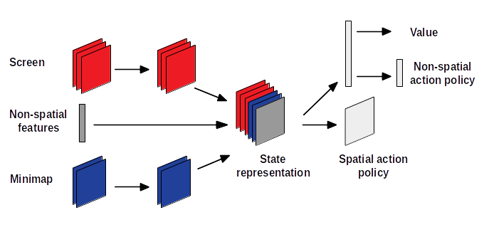
Figure 1 gives a schematic overview of the agent's architecture. The features of screen and minimap are extracted using two convolutional neural networks each. As mentioned above three features from the screen and two from the minimap are used. The output of the last convolutional neural networks is concatenated with the the oupput of a fully connected neural network that was fed with the non-spatial inputs described above which gives the state representation. The state representation fed into a another convoluted neural network that gives the coordinates for a spatial action. The state representation is also fed into another fully connected neural network, which gives value of the current state, the same fully connected neural network is fed into another fully connected network that gives the non-spatial action.
The output of all neural networks is encoded in one-hot encoding, also the one that gives the coordinates for a spatial action. In this case the output layer of the neural network has a size of x × y and the coordinates for X and Y are calculated by getting the position of the highest output and performing an integer division by the size of y for the Y-coordinate and a modulo by the size of x for the X-coordinate.
The first convolutional neural network for the screen and the minimap has 16 output filters, a kernel size of 5 and a stride of 1, the second one has 32 output filters, a kernel size of 3 and a stride of 1. The fully connected neural network for the non-spatial features has 256 outputs with tanh as activation function, the fully connected neural network for the state representation has 256 outputs with relu as activation function, the fully connected neural network for the non-spatial actions hast the number of available actions as output1 with softmax as activation function. The fully connected network for the value function has only one output and no activation function, since I am only interested in the value it returns.
The agent uses TensorFlow 1.5 as library for machine learning, the convolutional and fully connected neural networks are from the contrib.layers sub-module, contrib features volatile and experimental code, contrib.layers features more higher level operations for building neural networks.
In order to be able to run the algorithm on a regular laptop2, a few tweaks and reductions in complexity of the environment had to be made. The size of the screen and the minimap was reduced to 32 × 32. The agent was run in 16 parallel instances.
Algorithm
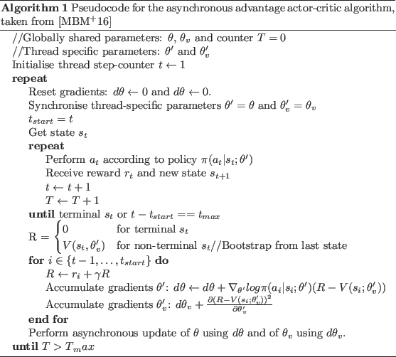
The asynchronous advantage actor critic algorithm (A3C) [MBM+16] was used as reinforcement learning algorithm. Its advantages are its simplicity, its efficiency as well as its performance. It is relative easy to implement and resource friendly, meaning that it doesn't require specialised hardware like GPUs to run efficiently3, but it still outperforms deep Q-learning on the Atari-domain and also succeeds in various continuous motor control tasks [MBM+16]. Previously deep reinforcement learning algorithms had problems with stability, deep Q-learning solved this problem by introducing a replay buffer [MKS+13], replay memory has the drawback of being quite resource consuming per real interaction Asynchronous approaches like A3C solve the problem of stability by introducing a parallel approach, the parallel execution and weight updates of different agent instances keeps the system stable.
A3C maintains a policy π(at | st; θ) and an estimate of the value function V(st;θv). In terms of actor-critic the policy is the actor and the estimate of the value function is the critic. Both get updated after every tmax steps performed by the agent4. The update of the neural network's weights can be described as ∇ θ' = log π(at | st; θ') A(st, at; θ, θ'), where A(st, ay; θ, θ') is an estimate of the advantage function given by Σi=0k-1 = γi rt+i + γk V(st+k ; θk) - V(st θ), where k is the number of the current state5 and is limited by tmax. The pseudocode for the algorithm is shown in algorithm 1.
Implementation of the Algorithm
Agent Step
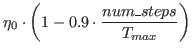
The algorithm for updating the weights is described in the section above. In every step the agent is fed with the above mentioned features from the screen, minimap and non-spatial features, in addition to the non-spatial features from the environment also whether the current availability from the executable actions is fed as input. The neural networks return the action to perform and the location where it should be performed. The output gets filtered, so that only a valid action (an action that the agent is currently able to do gets returned) gets passed on to the environment. During training there is a certain probability that the performed action is random or that the position where it performed is random. This level of randomness decreases depending on how many steps the agent has performed. The probability if an action is can be computed using this formula:
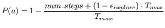
Where εexplore = 0.4 and Tmax = 600 × 106 (the maximum amount of steps that the agent makes). In addition to this adaptive probability there exists a second chance for an action to be random: an ε-greedy exploration where ε = 0.05. This was implemented so that the agent keeps exploring, even when the adaptive exploration probability reaches 0, which happens after 240 × 106 steps. The total probability of a random action is:
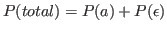
In the beginning (when numsteps = 0) this would be 0.4 + 0.05 = 0.45. The possibility of an position being random is computed using the same formula.
All the performed actions (with their positions) are stored, as well as the state for each step of the agent. The saved actions and states will be used for the training of the neural network as well as for logging the results of an episode with the actions the agent performed in this episode. In order to keep the size of the log files reasonable, only the actions for the top 10 episodes for minerals and gas, as well as the last 10 episodes are kept for every instance of the agent.
Update of the weights
After an episode finished, the weights of the neural networks are updated. The updates are done asynchronously, where each agent instance is contributing to the weights of the neural networks.
As described in section explaining the algorithm, first the cumulated rewards are calculated. For that list of rewards is initialised with either 0, when the episode reached a terminal state or the reward is bootstrapped from the last state. From that on the lists of performed actions and states are reversed and the rewards get cumulated by adding the sum of the last rewards multiplied by the discount factor6. By doing so the earlier the action took place, the higher the reward it gets assigned, given that the agent keeps on doing actions that give rewards. If the agent performs actions that decrease the rewards, also the reward decreases. The reward function is explained below.
The optimiser for updating the weights is the RMSPropOptimizer [HS17] with ε = 0.1 and decay = 0.99, the learning rate is variable and decreases the more steps the agent has performed. It can be calculated using the following formula:
Where η0 = 10-3 and Tmax = 600 × 106. The learning rate is fed into TensorFlow like an input for a neural network.
The other inputs that are fed are the states for each single step (screen, minimap and non-spatial features), the rewards for each single step, whether the selected action is spatial, which position was selected, which non-spatial actions are valid for the current state (this depends on which units are currently selected), which non-spatial action is selected and the learning rate. The variables for whether an action is spatial and valid non-spatial actions are used to create a mask for the computations of the logarithmic probability of an action.
One episodes consists of 840 steps, in which actions are performed7. In order to not need more memory for the updating of the weights than my GPU provides, I had to split the input data into 20 batches, where each includes number of 42 states, used as input.
After every 500 episodes, once the updating of the weights is done, the current weights are saved to hard disk.
Reward Function
The reward function for each step is:

The variables minerals and gas donate the totally collected amount of minerals and gas, minerals_rate and gas_rate denote the current collection rates of minerals and gas.
I gave gas a higher value than minerals, because minerals are rather straight forward to collect (the agent only has to select a worker unit and give the harvest command on a mineral field), while collection gas is much more complicated (the agent has to select a worker unit and then give a command to build a refinery on a specific field where a geyser is, in order to increase the collection rate of gas the agent can send more worker units to the build refinery).
I also decided to multiply the collection rate of both resources by the factor $ 10$ so that the collection rates are having significant influence on the total reward, also when the total collected amount of resources is already high.
Bibliography
BE17 Inc. Blizzard Entertainment.
SC2API documentation. https://blizzard.github.io/s2client-api/, 2017.
[Online; accessed 2018-03-29].HS17 Srivastava Nitish, Geoffrey Hinton and Kevin Swersky.
Lecture 6a overview of mini-batch gradient descent.
http://www.cs.toronto.edu/~tijmen/csc321/slides/lecture_slides_lec6.pdf, 2017. [Online; accessed 2018-03-29].MBM+16 Volodymyr Mnih, Adria Puigdomenech Badia, Mehdi Mirza, Alex Graves, Timothy Lillicrap, Tim Harley, David Silver, and Koray Kavukcuoglu.
Asynchronous methods for deep reinforcement learning.
In International Conference on Machine Learning, pages 1928-1937, 2016.MKS+13Volodymyr Mnih, Koray Kavukcuoglu, David Silver, Alex Graves, Ioannis Antonoglou, Daan Wierstra, and Martin Riedmiller.
Playing atari with deep reinforcement learning.
arXiv preprint arXiv:1312.5602, 2013.
Footnotes
1 Which is 15, as described above.
2 The agent was run on my laptop, which has an i7-7700HQ CPU, 16GB RAM, a GeForce GTX 1050 with 4GB of VRAM.
3 When run on such specialised hardware it of course drastically speeds up the computation.
4 In my implementation I perform an update after an episode finishes, so tmax = 840.
5 In my case this is equal to the number of the current step.
6 The discount factor γ is set to 0.99, because I am interested in the long term results of an action.
7 The execution of a map stops after 6720 steps, so for the environment it is actually 6720 steps, but since the agent only executed every 8th step, it only performs 840 actions.
Again, you scooped up useful information. Thank you author
d'U wanna defeat automaton 2000?)
It would have been nice, but my main focus was that the bot learns to gather resources without any "prior knowledge", so I didn't gave it any explicit instructions, I only gave it rewards for "good" actions.
My bot does around 180 APM, so it roughly emulates an advanced human player and has more focus on developing strategies instead of spamming actions.
forgot to resteem Ur brilliant post) keep on going!) I'm playing only with ai, 'cause of no skills, but I love watch some streams and championships)
Thank you :)
One thing I learned in this project was how to play StarCraft II, but I also only played against the AI, because I'm not sure how well my skills were in comparison with other players. Since I'm done now I guess I should give it a try.
beat them all on korean ladder?)
Ahahaha no, I guess that I seriously lack in skill for that.