Google matrix and PageRank
PageRank algorithm proposed by the cofounders of Google, Sergei Brin and Larry Page along with Rajeev Motwani and Terry Winograd till date remains as one of the most popular algorithms. It was used by Google to rank pages in the past. In this short article let us try and understand how it is calculated and how it is motivated.
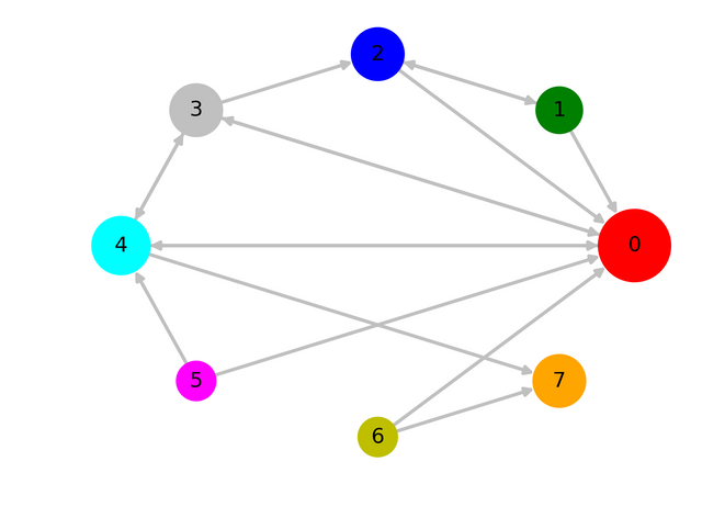
Fig-1 : Sample directed network with 8 nodes (source : created by me using matplotlib)
At the heart of PageRank algorithm lies the calculation of a matrix called the Google matrix. Google matrix is a Stochastic matrix (same as Markov matrix and Transition matrix). Given a network of webpages where there exists a edge from webpage i to webpage j if there is a hyperlink from webpage i to webpage j. This network of webpages in general is a directed network i.e. existence of an edge from i to j doesn't imply existence of an edge from j to i for any arbitrary i and j. We can represent this directed network using an Adjacency matrix A of dimensions N x N, where N is the total number of nodes (webpages in this case) in the network. A~ij~ = 1 if there exists a link from page j to page i. The Google matrix,G is calculates as suggested by the formula below,
Here S is matrix obtained from the adjacency matrix A by dividing each column of the adjacency matrix by the corresponding column's sum. In case of columns that have all zeros (i.e. corresponding to webpages that have no hyperlinks to any other pages), we replace all the elements of that column by 1/N. I is a N x N matrix with all elements equal to 1. alpha is a variable parameter that assigns weights to matrix S and I/N.
Stochastic matrices contain probabilities corresponding to transition from state j to state i. By their very definition all the columns sum to 1, since probability of transitioning from state j to any of the total N number of states is 1. While constructing the matrix S we divided the columns of the adjacency matrix by their corresponding sums (i.e. in-degrees). If j^th^ column has k non-zero (=1) values then these values are replaced by 1/k, meaning there is an equal probability of *1/k for going from j^th^ webpage to one of the k webpages to which the j^th^ webpage provides a link. In the case where j^th^ webpage had no links from it to any other webpage we assigned a probability of 1/N to go from j^th^ page to any of the total number of N pages.
If we were to consider a "surfer" starting at some webpage and randomly clicking on one of the links the current webpage contains and so on. In the absense of any such link the "surfer" randomly picks one of the N webpages that are available. This would be the dynamics described by the stochastic matrix S. On the other hand I/N describes a dynamics where the surfer at every instant just randomly jumps to one of the N webpages available. The matrix G describes a hybrid dynamics where at every instant with probability alpha the "surfer" moves according to S and with probability 1-alpha describes completely random hopping as described by I/N. We are interested in knowing after a long time how much of the total time is spent by our "surfer" at each of the N webpages. The eigenvector corresponding to the largest eigenvalue of the matrix G essentially provides the solution. The largest eigenvalue is always equal to 1 for G. Since the G matrix is assymetric the eigenvalues are in general complex. The reason for adding the stochastic part with the weight 1-alpha while constructing G is to ensure there is one unique eigenvalue with value equal to 1. alpha also impacts the value of the second largest eigenvalue and this is important since the ratio of the second largest eigenvalue to that of first largest eigenvalue (=1) determines how fast one can obtain the largest eigenvector from the Google matrix using Power Iteration procedure. Fig-4 shows the dependence of the magnitude of second largest eigenvalue on the value of alpha. The magnitude of second largest eigenvalue is smaller or equal to 1-alpha.
I will illustrate the above procedure on a made-up directed network in Fig-1
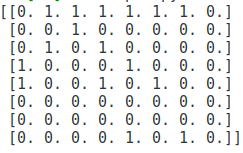
The adjacency matrix for the above matrix is,
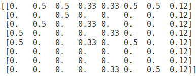
and the matrix S is,
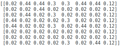
and the Google matrix, G for alpha = 0.85 is,
The top panel of the below figure shows the eigenvalue spectrum for the Google matrix, G calculated for the above network. The bottom panel shows each of the component of the eigenvector corresponding to the largest eigenvalue( blue circle in the top panel), which are essentially the PageRank value corresponding to each of the node in the above network.
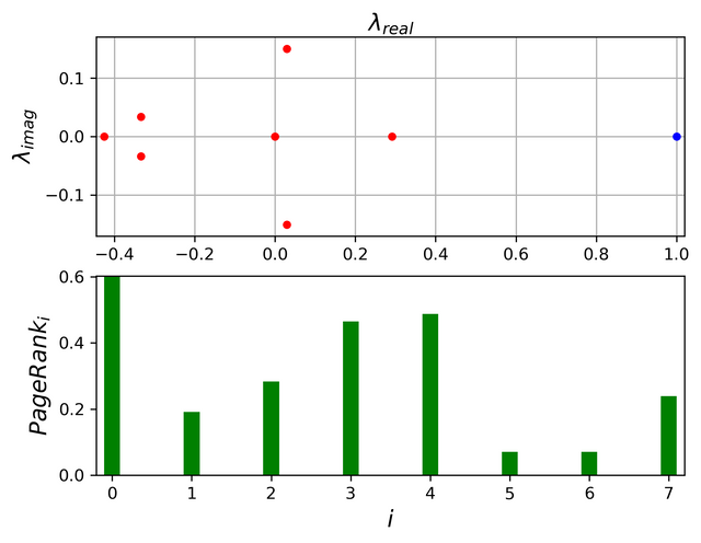
Fig-2 : Eigen spectra and the PageRank obtained for the above Network (source : created by me using matplotlib)
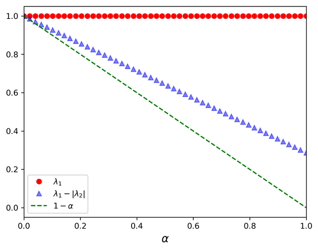
Fig-3 : Dependence of magnitude of second largest eigenvalue on the value of alpha. (source : created by me using matplotlib)
Wikipedia vote network
In order to illustrate the procedure on a real world network, I obtained the directed network of Wikipedia voting network constructed based on who has voted for whom in the "election" for an user to be promoted to the status of administrator. More information about the dataset can be obtained from here. The final directed network has 7066 nodes and 103663 edges. The reason for not using networks corresponding to actual webpages is the massive size of real world web networks. But the data can be found here.
The top panel of the below figure shows the eigenvalue spectra where the largest eigenvalue is shown in blue. The bottom panel shows the components corresponding to the largest eigenvector, which assigns the PageRank to each node.
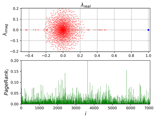
Fig-4 : Eigen spectra and the PageRank obtained for the Wikipedia Vote Network (source : created by me using matplotlib)
Typically alpha=0.85 is good choice where quick convergence is guaranteed for Power Iteration while avoiding degenerate eigenvalues equal to 1. The following figure illustrates how the convergence occurs with increasing number of iterations.
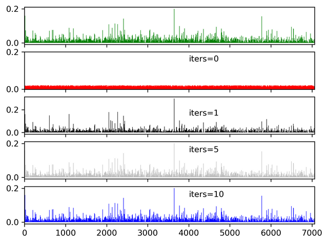
Fig-5 : Convergence of an uniform random vector to largest eigenvector when iteratively multiplied by the Google matrix with alpha=0.85 (source : created by me using matplotlib)
Relevant Python Code
Code related to the made up network
import pandas as pd
import numpy as np
import networkx as nx
import matplotlib.pyplot as plt

#-------- Code related to the made up network ------------#
def Sample_Graph(alpha=0.85):
    G = nx.DiGraph()
    N = 8
    G.add_nodes_from(range(N))
    Edges = [(1,0),(1,2),(2,1),(2,0),(3,2),(3,0),(0,3),(3,4),(4,3),(4,0),(0,4),(5,4),(5,0),(6,0),(6,7),(4,7)]
    G.add_edges_from(Edges)
    A = nx.to_numpy_array(G)
    A = A.T
    S = np.zeros(A.shape)
    for j in range(N):
        k = np.sum(A[:,j])
        if k > 0:
            S[:,j] = A[:,j]/k
        else:
            S[:,j] = 1.0/N
    Google = alpha*S + (1-alpha)*(np.ones(S.shape)/N)
    [E,V] = np.linalg.eig(Google)
    idx = np.abs(E).argsort()
    E,V = E[idx],V[:,idx]

    #========================== Visualization ================================#
    Sz = [500+G.in_degree[i]*200 for i in range(8)]
    POS = nx.circular_layout(G)
    COL = ['r','g','b','silver','cyan','magenta','y','orange']
    fig,ax = plt.subplots()
    nx.draw_networkx(G,pos=POS,node_size=Sz,ax=ax,node_color=COL,edge_color='silver',width=2)
    ax.axis('off')
    plt.savefig('Sample_Net.png',dpi=300,bbox_inches='tight')
    plt.close()

    xmin,xmax = np.min(E.real),np.max(E.real)
    ymin,ymax = np.min(E.imag),np.max(E.imag)
    fig,ax = plt.subplots(nrows=2)
    ax[0].plot(E.real[:-1],E.imag[:-1],'ro',alpha=1.0,markersize=4)
    ax[0].plot(E.real[-1],E.imag[-1],'bo',alpha=1.0,markersize=4)
    ax[0].set_xlim(xmin-0.02,xmax+0.02)
    ax[0].set_ylim(ymin-0.02,ymax+0.02)
    ax[0].set_xlabel(r'$\lambda_{real}$',fontsize=14)
    ax[0].xaxis.set_label_position('top')
    ax[0].set_ylabel(r'$\lambda_{imag}$',fontsize=14)
    ax[0].grid('on')
    #------------------------------------------------#
    Z = V[:,-1].real
    #ax[1].vlines(range(len(Z)),ymin=0,ymax=Z,colors='g',linewidth=0.5)
    ax[1].bar(range(len(Z)),Z,color='g',width=0.2)
    ax[1].set_xlim(0-0.2,len(Z)-0.8)

    ax[1].set_ylim(0,np.max(Z))
    ax[1].set_xlabel(r'$i$',fontsize=14)
    ax[1].set_ylabel(r'$PageRank_i$',fontsize=14)
    plt.savefig('Sample_Spectrum.png',dpi=300,bbox_inches='tight')
    plt.show()
    #==============================================================#
    return(G)
Code related to the Wikipedia Vote Network
import pandas as pd
import numpy as np
import networkx as nx
import matplotlib.pyplot as plt

def Gen_Google_Matrix(A,alpha=0.85):
    N = A.shape[0]
    S = np.zeros(A.shape)
    K = np.sum(A,0)
    idx = np.nonzero(K == 0)[0]
    S[:,idx] = 1.0/N
    idx = np.nonzero(K)[0]
    K = K[idx]
    A = A[:,idx]
    S[:,idx] = A/K[None,:]
    G = alpha*S + (1-alpha)*(np.ones(S.shape)/N)
    return(G)

def Construct_Graph():
    df = pd.read_csv('Wiki-Vote.txt',sep='\t')
    Source,Sinks = np.array(df.Source),np.array(df.Sink)
    N = max(np.max(Source),np.max(Sinks))
    Source,Sinks = Source-1,Sinks-1
    G = nx.DiGraph()
    G.add_nodes_from(range(N))
    G.add_edges_from(list(zip(Source,Sinks)))
    G = max(nx.weakly_connected_component_subgraphs(G),key=len)
    A = nx.to_numpy_array(G)
    Google = Gen_Google_Matrix(A.T,0.85)
    [E,V] = np.linalg.eig(Google)
    idx = np.abs(E).argsort()
    E,V = E[idx],V[:,idx]
    np.save('Wiki_Lambdas.npy',E)
    np.save('Wiki_LargestEigenVec.npy',V[:,-1].real)
    return(A)

#------------ Visualizing the saved numpy arrays --------------#

E = np.load('Wiki_Lambdas.npy')
Z = np.load('Wiki_LargestEigenVec.npy')
xmin,xmax = np.min(E.real),np.max(E.real)
ymin,ymax = np.min(E.imag),np.max(E.imag)
fig,ax = plt.subplots(nrows=2)
ax[0].plot(E.real[:-1],E.imag[:-1],'ro',alpha=0.3,markersize=2)
ax[0].plot(E.real[-1],E.imag[-1],'bo',alpha=1.0,markersize=4)
ax[0].set_xlim(xmin,xmax+0.02)
ax[0].set_ylim(ymin,ymax)
ax[0].set_xlabel(r'$\lambda_{real}$',fontsize=14)
ax[0].xaxis.set_label_position('top')
ax[0].set_ylabel(r'$\lambda_{imag}$',fontsize=14)
ax[0].grid('on')
#------------------------------------------------#
ax[1].vlines(range(len(Z)),ymin=0,ymax=Z,colors='g',linewidth=0.5)
ax[1].set_xlim(0,len(Z)-1)
ax[1].set_ylim(0,np.max(Z))
ax[1].set_xlabel(r'$i$',fontsize=14)
ax[1].set_ylabel(r'$PageRank_i$',fontsize=14)
plt.savefig('Wiki_Spectrum.png',dpi=300,bbox_inches='tight')
plt.show()
Dependence of alpha
def Alpha_Dependence():
    G = nx.DiGraph()
    N = 8
    G.add_nodes_from(range(N))
    Edges = [(1,0),(1,2),(2,1),(2,0),(3,2),(3,0),(0,3),(3,4),(4,3),(4,0),(0,4),(5,4),(5,0),(6,0),(6,7),(4,7)]
    G.add_edges_from(Edges)
    A = nx.to_numpy_array(G)
    Alphas = np.linspace(0.0,1.0,50)
    L1,L2 = np.zeros(50),np.zeros(50)
    for i in range(len(Alphas)):
        alpha = Alphas[i]
        GM = Gen_Google_Matrix(A,alpha)
        [E,V] = np.linalg.eig(GM)
        idx = np.abs(E).argsort()
        E,V = E[idx],V[:,idx]
        L1[i],L2[i] = np.abs(E[-1]),np.abs(E[-2])
    fig,ax = plt.subplots()
    ax.plot(Alphas,L1,'ro',label=r'$\lambda_1$')
    ax.plot(Alphas,L1-L2,'b^',label=r'$\lambda_1-|\lambda_2|$',alpha=0.5)
    ax.plot(Alphas,1-Alphas,'g--',label=r'$1-\alpha$')
    ax.legend(loc='best')
    ax.set_xlim(0,1)
    ax.set_xlabel(r'$\alpha$',fontsize=14)
    plt.savefig('Alpha_Dependence.png',dpi=300,bbox_inches='tight')
    plt.show()
Method of Power Iteration
def Power_Iteration(G,iters=[0,1,5,10]):
    N = G.shape[0]
    L = np.random.rand(N)
    D = np.zeros((len(iters),N))
    idx = 0
    for i in range(max(iters)+1):
        if i in iters:
            D[idx,:] = L
            idx += 1

        L = G.dot(L)

    return(D
#============= plotting the convergence ==============#
Z = np.load('Wiki_LargestEigenVec.npy')
G =  Construct_Graph()
G = scipy.sparse.csr_matrix(G)
D = Power_Iteration(G)
L1,L2,L3,L4 = D[0,:]/np.linalg.norm(D[0,:]),D[1,:]/np.linalg.norm(D[1,:]),D[2,:]/np.linalg.norm(D[2,:]),D[3,:]/np.linalg.norm(D[3,:])
fig,ax = plt.subplots(nrows=5,sharex=True)
ax[0].vlines(range(len(Z)),ymin=0,ymax=Z,colors='g',linewidth=0.5)
ax[1].vlines(range(len(L1)),ymin=0,ymax=L1,colors='r',linewidth=0.5)
ax[2].vlines(range(len(L2)),ymin=0,ymax=L2,colors='k',linewidth=0.5)
ax[3].vlines(range(len(L3)),ymin=0,ymax=L3,colors='silver',linewidth=0.5)
ax[4].vlines(range(len(L4)),ymin=0,ymax=L4,colors='b',linewidth=0.5)
ax[0].set_yticks([0,0.2])

ax[1].set_yticks([0,0.2])
ax[2].set_yticks([0,0.2])
ax[3].set_yticks([0,0.2])
ax[4].set_yticks([0,0.2])

ax[1].text(4000,0.15,'iters=0')
ax[2].text(4000,0.15,'iters=1')
ax[3].text(4000,0.15,'iters=5')
ax[4].text(4000,0.15,'iters=10')
ax[4].set_xlim(0,len(Z)-1)
plt.savefig('Convergence.png',dpi=300,bbox_inches='tight')
plt.show()
References
- Page, L., Brin, S., Motwani, R., & Winograd, T. (1999). The PageRank citation ranking: Bringing order to the web. Stanford InfoLab.
- https://en.wikipedia.org/wiki/PageRank
- https://en.wikipedia.org/wiki/Stochastic_matrix
- https://en.wikipedia.org/wiki/Google_matrix
- https://en.wikipedia.org/wiki/Power_iteration
- http://www.scholarpedia.org/article/Google_matrix
- https://snap.stanford.edu/data/wiki-Vote.html
- J. Leskovec, D. Huttenlocher, J. Kleinberg. Signed Networks in Social Media. CHI 2010.
- J. Leskovec, D. Huttenlocher, J. Kleinberg. Predicting Positive and Negative Links in Online Social Networks. WWW 2010.
- http://latex2png.com/ (for exporting latex eqs to png files)

Great research and nice level of details.
Thanks!
Congratulations @boyonpointe! You received a personal award!
You can view your badges on your Steem Board and compare to others on the Steem Ranking
Vote for @Steemitboard as a witness to get one more award and increased upvotes!