Fooling around with Self Organizing Maps (SOM)
Couple of months back while working on some PhD problem of mine I realized I would be needing some way to visualize data that is of dimensions higher than 3. Googling in the hope of some solutions lead me to an obscure geological research paper which made use of Self Organized Maps.My first impression of it was good enough to pursue it further. Eventually after some amount of exploration, I felt it was time to share what I learnt in the past month or so.

Introduction
SOMs were introduced in 1982 by a Finnish professor named Teuvo Kohonen in a paper published in the journal, Biological Cybernetics [1]. To use the Machine Learning jargon, SOM is an unsupervised learning method. It is primarily used for visualizing higher dimensional data by projecting them onto 2D or 1D grid. Data points that are closer in the original dimension remain closer in SOM grid,as in the original distance relationships are preserved.
Let us consider M data points in d dimensional space. We can represent these M data points as M d dimensional vectors. We also need a meaningful metric in d dimensional space in order to talk about distance between any pair of d dimensional vectors. Very often the Euclidean norm,
serves as a good metric. v,w are two vectors in d dimensional space. The objective of SOM is to map these M d dimensional vectors onto a 1D or a 2D grid. SOM ensures that two vectors that are closer in d dimensional space remain closer in the reduced dimensional space as well, thereby ensuring that the topological properties are preserved.
Implementation
The common method through which SOM implementation is explained is what is called Stepwise recursive algorithm. One starts off by defining a 1D or a 2D grid with N grid points, hereafter lets just assume we are considering a 2D grid. Let n_rows and n_cols be the number of rows and columns of the 2D grid then N is simply, N = n_rows * n_cols. We assign a random vector to each of these N grid points. We need to also define a neighborhood function,
hij spits out the amount of "impact" grid vector vj has on the grid vector vi and this is a function of the distance between the two vectors in 2D space and the "time", t. By time here I mean the iteration number or something similar. In the case of Stepwise recursive algorithm it refers to the iteration number. Typically hij is a monotonically(weakly) decreasing function of L2 and t.
We pick one random data vector, vr at a time from the M data vectors and calculate the distance between vr and the and all the N grid vectors. The grid vector which is closest to vr is said to be the winning vector vw. Once we find out the vw for a given vr we then make the the grid vector vw orient a bit more in the direction of the data vector vr. We don't just stop there but we make all the neighbors of the vector vw orient a bit more in the direction of vr. The set of vectors that comprise the neighborhood of vw and the amount of change these neighbors undergo is obtained by the neighborhood function hwr. In general grid vectors that are closer to vw undergo more change than the ones that are further away. And a given vector in the neighborhood undergoes more change in the beginning than towards the end since neighborhood function is a monotonically decreasing function of t as well as the distance.
The above expression is an example of typical neighborhood function [2]. g(t) needs to be a monotonically decreasing scalar function of t and distance L2 between the vw and vj on the 2D grid. The exact form of g(t) is not so important and it can be hyperbolic, exponential, piecewise linear etc and some of them might work better than others in specific contexts. After a large number of iterations the grid vectors will converge to their asymptotic directions (at least that is the hope).
Once the above process is done we can obtain the exact mapping between each of the M data vector and N grid vectors. One can now obtain a 2D histogram based on the number of data vectors that have been mapped onto each of the N grid vectors. If we happen to have chosen not too few nor not too many grid vectors we might see clusters in the histograms, as in groups of grid vectors separated by grid vectors that have no or very few data vectors mapped on to them. In this way one can use the histograms obtained for de novo cluster prediction. There are no good thumb rules (at least that I am aware of) as to what qualifies as a good value of N. Typically one needs to try out various different values and finally use the one that makes sense. Simply put there are no hard and fast rules and the choice of N should stem from something inherent to the data which hopefully the user is aware of !
The batch computation algorithm
Though stepwise recursive algorithm is widely used to elucidate the principle of SOM, when it comes to actually implementing people very often use the batch computation algorithm. The reason for it being that higher level languages and libraries like MATLAB, Python(Numpy, Scipy ...), R lets you calculate large distance matrices in very little time. In principle both the algorithms should converge to the same final state or at least very similar. I wont focus on these aspects since I am ignorant of all the theory behind these algorithms and I am mostly interested in being able to implement these in order to solve problems. Interested people can find plenty of references by going through the review article by Kohonen in 2013 [2].
In case of the batch computation method you don't pick one vector at a time from M vectors instead you start by calculating distance matrix D of dimensions M * N between the M data vectors and N grid vectors. From this matrix you obtain the list of all data vectors that have been mapped on to each of the grid vectors. Its completely normal to have empty list for some of the grid vectors. Once this is done you update the position of all the N vectors in one shot! In order to do this one has to get the union of all the lists of data vectors that have been mapped on to a particular grid vector and it's neighbors. Let's say the grid vector of interest is vw and at a given time t it has 4 neighbors va,vb,vc,vd. We also know the lists of data vectors that have been mapped on to these vectors. Our task involves calculating,
Since each data vector will be mapped onto an unique grid vector the above union operation is done over disjoint sets. Once LU is obtained you update the vector Lw by the mean vector calculated by summing all the vectors in LU component wise and dividing it by the number of vectors in LU (i.e. cardinality of LU). In the case of this method at the end of an iteration all the grid vectors are updated. Usually few tens of iterations are good enough. Another great thing about this method is one need not break their head over learning rates. But it is true that one can obtain weighted mean of vectors in the neighborhood instead of being very democratic.
Where is the code dude ?
The following is the complete code that I wrote in Python to implement batch method. I have used a very simple function for the neighborhood size, it basically decreases from rmax to rmin with t, t being the number of times I have updated the grid vectors. The total number of times I update the grid vectors is specified by the parameter nepochs.
from __future__ import division

import numpy as np
from matplotlib import pyplot as plt
import pandas as pd
import time
import copy
from PIL import Image
import scipy.spatial.distance as ssd
from matplotlib import colors

class SelfOrganizingMap(object):

    def __init__(self,nrows,ncols,rmin=None,rmax=None):
        self.nrows      = nrows
        self.ncols      = ncols

        if ((nrows > 1) and (ncols > 1)):
            self.dimension = 2
        else:
            self.dimension = 1

        self.diameter   = max(nrows,ncols)
        self.hungry     =  True
        self.n_gridvecs = nrows*ncols
        if rmax == None:
            self.rmax = min(int(self.diameter/2.0),min(nrows,ncols))
        else:
            self.rmax = rmax

        if rmin == None:
            self.rmin = 1
        else:
            self.rmin = rmin


    def eat_this_data(self,data):
        self.data   = data
        self.nvecs  = data.shape[0]
        self.vdim   = data.shape[1]
        self.hungry = False

    def setup_grid(self):
        IDX        = np.random.randint(0,self.nvecs,self.n_gridvecs)
        #self.grid  = np.random.random((self.n_gridvecs,self.vdim))
        self.grid  = self.data[IDX,:]
        if self.dimension == 2:
            Location   = np.zeros((self.n_gridvecs,2))
            for k in range(self.n_gridvecs):
                Location[k,:] = [k//self.ncols,k%self.ncols]
            self.GD = ssd.squareform(ssd.pdist(Location,metric='chebyshev'))
        else:
            Location = np.arange(self.n_gridvecs).reshape((self.n_gridvecs,1))
            self.GD = ssd.squareform(ssd.pdist(Location,metric='chebyshev'))

    def get_dist_array(self):
        dist_array = ssd.cdist(self.data,self.grid)
        return(dist_array)

    def get_radius(self,epoch):
        e_lambda= np.log(self.rmax/self.rmin)/(self.nepochs-1)
        radius  = self.rmax * np.exp(-e_lambda*epoch)
        return(radius)

    def get_1D_neighbors(self,idx,rad):
        neighbors = np.nonzero(self.GD[idx,:] <= rad)[0]
        return(neighbors)


    '''
    NIDX[j,:n_inf] : union of all data vectors mapped on to the node j and it's neighbors
    '''
    def get_influencers_list(self,rad):
        D    = self.get_dist_array()
        NIDX = np.zeros((self.n_gridvecs,self.nvecs),dtype=int)
        NInf = np.zeros(self.n_gridvecs,dtype=int)
        Z    = np.argmin(D,axis=1)
        for j in range(self.n_gridvecs):
            neighbors = self.get_1D_neighbors(j,rad)
            matches   = np.isin(Z,neighbors)
            NInf[j]   = np.sum(matches)
            NIDX[j,:NInf[j]] = np.nonzero(matches)[0]
        return(NIDX,NInf)


    #------------------------------------------------------------#
    def train_grid(self,nepochs):
        self.setup_grid()

        self.nepochs     = nepochs

        tot_changes = []

        for epoch in range(nepochs):
            print('epoch = '+str(epoch))
            new_grid = np.random.random((self.n_gridvecs,self.vdim))
            radius = self.get_radius(epoch)

            NIDX,NInf = self.get_influencers_list(radius)

            for idx in range(self.n_gridvecs):
                if NInf[idx] == 0:
                    new_grid[idx,:] = copy.deepcopy(self.grid[idx,:])
                else:
                    new_grid[idx,:] = np.mean(self.data[NIDX[idx,:NInf[idx]]],axis=0)

            delta = np.sum(np.abs(new_grid-self.grid))

            tot_changes.append(delta)
            self.grid = copy.deepcopy(new_grid)
        #---------------------------------------------------------#
        D = self.get_dist_array()
        B = np.argmin(D,axis=0)

        Z = np.argmin(D,axis=1)
        NW = np.array([np.count_nonzero(Z==node) for node in range(self.n_gridvecs)])

        print(NW,np.count_nonzero(NW))

        fig,ax = plt.subplots()
        ax.plot(range(nepochs),tot_changes,'ro')
        ax.set_xlabel('epochs')
        ax.set_ylabel(r'$\delta$')
        plt.show()

        return(self.grid,B,NW)
    #-------------------------------------------------------------#
The "Hello, World" of SOMs
The most common example used to demonstrate how vectors that are closer in original d dimensions remain closer in lower dimension is by making use of 3D RGB vectors and projecting them onto a 2D grid. This is a nice example because human eyes are pretty good at noticing colors that are close to each other. This example involves sampling a large number of 3D vectors which have values between 0-255. Each of the three dimensions correspond three basic color intensity. And here is the code,
def Color_Data():
    Data = np.random.randint(0, 255, (10000,3))
    #--- uncomment to sample only shades of red --#
    #Data[:,1] = 0.0
    #Data[:,2] = 0.0

    Data = Data/255.0 #normalization
    nrows,ncols = 10,10
    nepochs = 100
    som = SelfOrganizingMap(nrows,ncols)
    som.eat_this_data(Data)
    G,B,NW   = som.train_grid(nepochs)

    Img = np.zeros((nrows,ncols,3),'uint8')
    for i in range(nrows):
        for j in range(ncols):
            k = i*ncols + j
            Img[i,j,0] = G[k,0]*256
            Img[i,j,1] = G[k,1]*256
            Img[i,j,2] = G[k,2]*256

    Img = Image.fromarray(Img)
    plt.imshow(Img,interpolation='nearest')
    plt.axis('off')
    #plt.savefig('colors_red.png',dpi=300,bbox_inches='tight')
    plt.show()
In the above code I sample 10000 colors and display them on a 10*10 grid. And I use batch method to train my SOM grid vectors, since each of the grid vector is also a 3D color vector I can assign RGB value to each of the final 100 grid vectors and display it as an image. And here is how it looks,
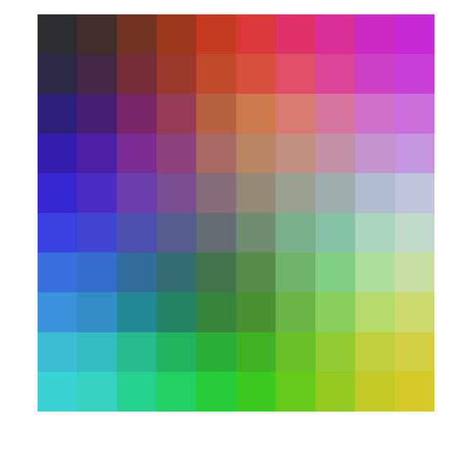
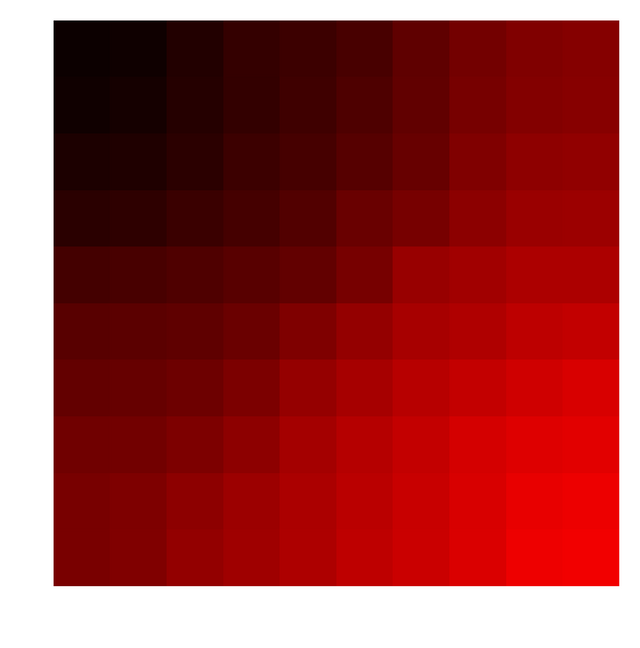
One can clearly see how closer colors are arranged closer to each other on a 2D grid. Just for fun one can uncomment the few lines in the above function and sample colors for which Green and Blue intensities are zero. Or in other words sample just shades of pure red and do the same thing as above. Here is what you end up with,
Show me some results
I obviously tried this on the famous Iris dataset. The data contains 150 3D vectors and there are 50 each flowers belonging 3 different species (setosa, versicolor, virginica).
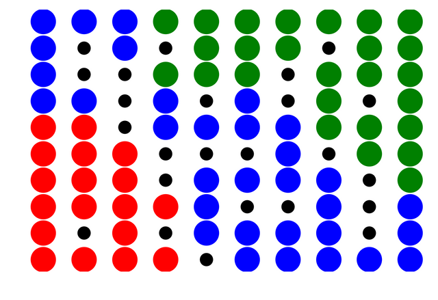
The blue,green and red circles represent grid vectors which have $>0$ of data vectors mapped onto them and their color is obtained based on the color of the data vector the each grid vector is closest to. Black circles indicate grid vectors no data vectors mapped onto them.
MNIST dataset
MNIST is a famous dataset that contains 60,000 $28\times28$ grayscale images with pixel values between 0-255 of hand written digits (0-9). The kaggle dataset has split this 60,000 into 42,000 + 28,000 images. 42,000 is the training set with 784 pixel values and corresponding label. I used 42,000 images to obtain SOM. I chose 50*50 grid to map the 784 dimensional vectors. I initialized the initial grid vectors using random 2500 data vectors.
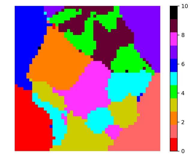
I did the same exercise but instead of retaining the grayscale value I converted the images to binary images. I made all non-zero grayscale values equal to 1. The results obtained were pretty similar. Note that two runs of SOM code produces different looking visualization because of the random initial conditions for the grid vectors. Here is the figure corresponding to binarized data,
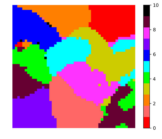
In both the images the color black is used to indicate grid vectors with no data vectors mapped onto them. Almost all vectors out of 2500 vectors had some vectors mapped onto them, so in order to obtain boundaries between the clusters using the histogram one needs to take more grid vectors (may be 80 * 80 or 100 * 100). In any case for 50*50 for a particular run the histogram looked like this,
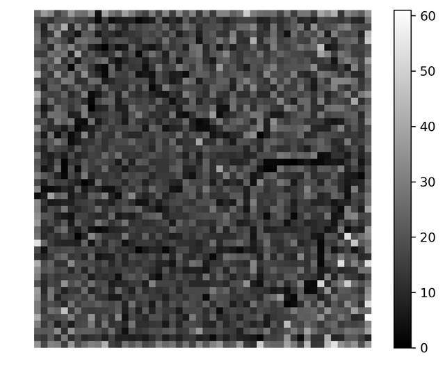
I wouldn't say the above histogram would be very handy in finding clusters but I feel larger system should do better.
Making predictions with SOMs
Though SOMs are primarily used for visualizing higher dimensional data, one can use it as a prediction tool as well. In the case of MNIST data the test set contains 28,000 images whose identity/label is not revealed. Once you obtain the SOM, one can for every unlabeled image obtain the grid vector that is closest to it and since we know the mapping between every grid vector and digits between 0 to 9, one can predict the label of the unlabelled image. I used SOMs obtained for grayscale and binarized images to label the unlabelled data and submitted to Kaggle MNIST challenge. Both of them predicted ~92% labels accurately with the binary one doing better ! 92% is a very respectable score for a tool that is primarily used for visualization.

I personally feel if I binarize the data in some more meaningful way the prediction quality might improve further. I hope this article will motivate more people to fool around with SOMs. Thank you for your time.
Note: Since steemit has no native mathjax support main equations had to be input as images. I made use of the website quicklatex for generating the images of the above equations.
References
[1] Kohonen, Teuvo. "Self-organized formation of topologically correct feature maps." Biological cybernetics 43.1 (1982): 59-69.
[2] Kohonen, Teuvo. "Essentials of the self-organizing map." Neural networks 37 (2013): 52-65.


Colleague, welcome to Steemit (I'm working in the field of chemometrics).
Ah... Iris dataset, alfa and omega...
Thank you :-)
Hi @boyonpointe!
Your post was upvoted by utopian.io in cooperation with steemstem - supporting knowledge, innovation and technological advancement on the Steem Blockchain.
Contribute to Open Source with utopian.io
Learn how to contribute on our website and join the new open source economy.
Want to chat? Join the Utopian Community on Discord https://discord.gg/h52nFrV
Sure. Thanks
So the original paper, since it was a geology paper, used this method in some relation to constructing literal geological maps?
Congratulations @boyonpointe! You have completed some achievement on Steemit and have been rewarded with new badge(s) :
Click on the badge to view your Board of Honor.
If you no longer want to receive notifications, reply to this comment with the word
STOPI have yet to take the time to really think through the math, but this seems very similar in its goal to the ordination techniques (often PCoA or NMDS) I use in ecology to represent the differences between communities on a 2D or 3D map. Very interesting.
Congratulations @boyonpointe! You have completed some achievement on Steemit and have been rewarded with new badge(s) :
Click on the badge to view your Board of Honor.
If you no longer want to receive notifications, reply to this comment with the word
STOPDo not miss the last announcement from @steemitboard!