Chapter 6 – Volatility

In short, volatility is the speed of change in the market. Markets that are slow are considered low-volatility. This section quantifies volatility.

Random Walks and Normal Distributions

Consider the game Plinko, if you remember it from The Price is Right. A ball is dropped down a series of uniformly placed pegs and the spot where it lands is the prize that the contestant wins. Natenburg describes this thoroughly. The ball has a 50/50 chance to turn right or left at each fork with 11 spots to drop into on the bottom (big money in the center). The reason the 10,000 is in the center is easy to explain because the number of left and right turns being equal is less likely!

Now, the reason he uses this example to describe volatility is that if you drop an infinite number of balls down the game it creates a bell curve. If you have ever taken Probability and Statistics this is common to you. We can apply this same bell curve to the underlying price of options contracts if we know the volatility allowing us to predict probability of success of a trade.

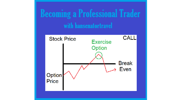
The higher the volatility the higher the value of an option contract because it has a much higher rate of success. Trading several thousand contracts with say a 70% win rate will make money just like a casino does it, with an edge.

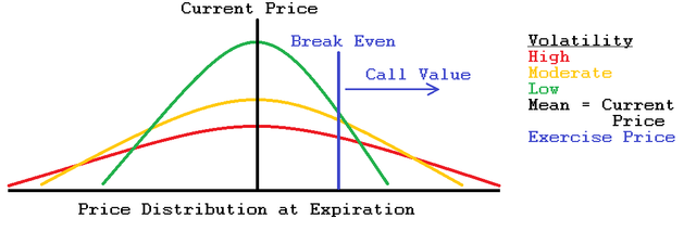
Volatility Model

Reference

Mean and Standard Deviation

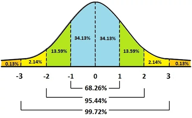
This Normal Curve above can be described by only two things, mean (μ) and standard deviation (σ). Our mean is the current underlying price. The standard deviation, σ, tells us how much of our data lays around the mean.
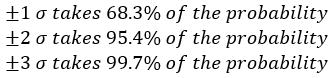
The normal curve above shows how the mean and standard deviation are related to it. Notice:

Example

Question: If our Plinko Board has a mean at 7.5 and a standard deviation of 3, what is the probability that a ball will drop lower than 5 or higher than 10?
Answer: Seeing that each drop can only be an integer our highest in 1 standard deviation is 10 and the lowest is 5, this is 68.3% of our probability, so 100 - 68.3 = 31.7% to be out of this range!

Forward Price as the Mean of a Distribution

Assuming that no arbitrage opportunity exists, we must assume the mean to be the forward price.

Volatility as a Standard Deviation

Volatility is a trader’s name for standard deviation, they mean the same thing. For now, we will assume that the volatility we feed into a pricing model represents a one standard deviation price change, in percent, over a one-year period.

Example:

Consider an option with a forward price of $100 and a volatility of 20%. This means that 68.3% probability of being between the two following numbers calculated.

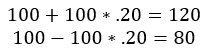
For two standard deviations we add and subtract 40 from 100 and that will tell us that 95% of our data will fall between 60 and 140. It’s a large range, but that is because of the high volatility of 20%.

Never Confuse Unlikely with Impossible!!! Spinning black on a roulette wheel 10-15 times in a row happens, not often.

Scaling Volatility for Time

There is a great equation for this section!

Traders can set time to weeks or days. There are 256 trading days in a year or 52 weeks.

Example

If the volatility of an option is 20% and a trader has 3 weeks to get rid of it, then the equation will be

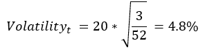
Thus, if the current price of the option is 100, then we can expect with a 68.3% confidence that the price will be between 95.2-104.8 in 3 weeks.

Volatility and Observed Price Changes

An earlier example in the text describes a 37% volatility for a 45-dollar forward price which was calculated for a daily change of $1.04 per day. The market reflects the following changes over the next week:

Does this reflect our calculated volatility? No, because the range should be a little higher than it is. Maybe the volatility is wrong? This is the reason a trader must consider observation prior to the trade to see if the volatility makes sense. Volatility is determined by settlement prices at the end of a day.

A Note on Interest-Rate Procedures

For some interest-rate products, primarily Eurocurrency interest-rate futures, the listed contract price represents the interest rate associated with that product, as a whole number subtracted from 100. So a 7% interest rate would be shown as 93.00.

Example:

A Eurodollar futures contract trading at 93.00 with a volatility of 26%, an approximate daily and weekly one standard deviation price change would be:

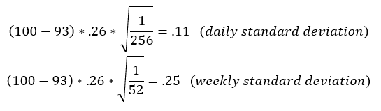
Note: A price change over 2 standard deviations will happen about 1 out of 20.

If we were to take a series of bond prices and from these calculate a series of yields, we could calculate the yield volatility, that is, the volatility based on the change in yield. You can use this to estimate the value of an option on a bond.

Lognormal Distributions

The normal distribution has a flaw. The belief in negative values of a stock price, so the lognormal distribution fixes that! Natenburg has defined volatility in terms of the percent changes in the price of an underlying instrument. In this sense, an interest rate and volatility are similar in that they both represent a rate of return. The primary difference between interest and volatility is that interest accrues only at a positive rate, whereas volatility is a combination of positive and negative rates of return.

A Simple Interest Example (easily calculatable):

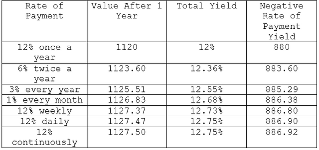
The Black-Scholes is a continuous-time model. It assumes that volatility is compounded continuously, just as if the price changes in the underlying contract, either up or down, are taking place continuously but at an annual rate corresponding to the volatility associated with the contract. When the percent price changes are normally distributed, the continuous compounding of these price changes will result in a longitudinal distribution of prices at expiration.

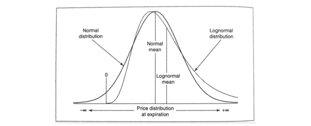
Notice that the mean of the lognormal distribution is higher that the normal mean. This is due to the larger tail on the right side caused by the non-negative values.

Example of Price Distributions:

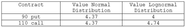
The value of the 110 call will be worth more value because it can potentially appreciate without limit because the price of the underlying contract has no limit on the upside. The 90 put can only rise to a max value of 90 because the price of the underlying contract can never fall below zero.

Interpreting Volatility and Data

Natenburg begins by dividing the volatility into two categories, realized volatility (for the underlying contract) and applied volatility (for options).

Realized Volatility

Realized Volatility is historical volatility based on time and fluctuation that has happened. This can give a trader valid insight on how a stock can preform in the future. Natenburg describes that it is also based on user input and mispriced stocks can be found based on opinion of the market. User input can tell historical volatility for 250-day, 52-week, or 12-month can all be slightly different and can affect decisions. A product that is volatile from day to day is equally as likely to be as volatile week to week or month to month.

Implied Volatility

Implied Volatility is the market’s consensus of what the future realized volatility of the underlying contract will be over the life of an option. We can use the Black-Scholes Equation to solve for volatility given interest rates, time to expiration, underlying price, etc. There are different forms of the model and it depends on which model you use because they can yield significantly different implied volatilities.

Solving for Theoretical Value Example

Traders are taught to sell overpriced options and buy underpriced options. Lets say a 105 call has a theoretical value of 2.94 and a price of 3.60, the 105 call is .66 overpriced. But in volatility terms the option is 3.50 volatility points overpriced because its theoretical value was based on a volatility of 25%, while its price is based on a volatility of 28.5% (the implied volatility). Given the unusual characteristics of options, it is often more useful to consider an option’s price in terms of implied volatility rather than total points.

Future realized volatility of an underlying contract determines the value of options on that contract. Implied volatility reflects an option’s price.

Traders use the words implied volatility and premium interchangeably because the implied volatility is derived from the option price and a higher volatility means a higher premium.

Natenburg describes prices and the importance of trading with volatility. I think of it as having a better edge for success. If volatility is low and the underlying price is low, then there is more than one way to profit. You want to buy calls and sell puts. It works in the other direction the same way!

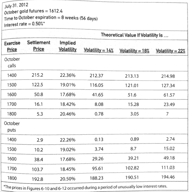
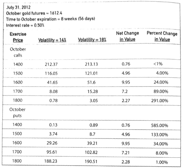
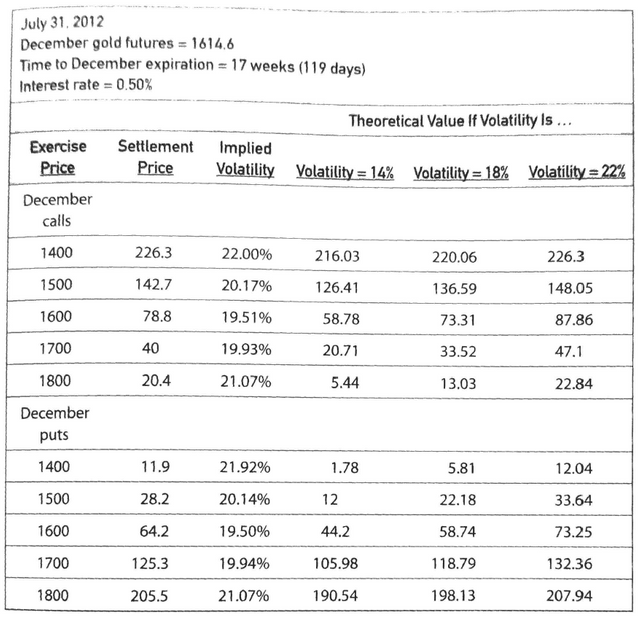
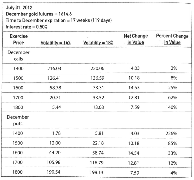
Gold Price Examples

Take a look at the prices and volatility to understand how they work:

Thank you for learning! Cheers & Best Wishes!