SEC | S20W2 | Data Analysis with Google Sheets: (Advanced Excel formulas, and pivot tables.)
Greetings Steemit friends
- Explain what you understand by Advanced Excel Formulas, and show us where advanced formulas such as the lookup function, and logical function are found in Excel with clear screenshots.
Advanced Excel Formulas, from the term advance, is an upgrade of the simple formulas we can find on Microsoft Excel. Advanced means the formula is made of multiple functions to obtain its objective. As I mentioned, advanced formulas af are more complex than the normal simple functions. Advanced formulas have proven to be more efficient in handling huge amounts of data collected.
Lookup function
The lookup function searches related data from a table and displays it more efficiently. The lookup function is best for data analysis and reporting accurate results while limiting common human errors. There are five lookup functions: Vertical Lookup, Horizontal Lookup, INDEX, MATCH, LOOKUP, and XLOOKUP. Lookup functions work best with an array of data.
Where to access the lookup function
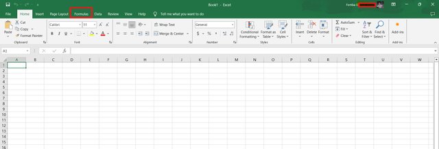
Launch the Microsoft Excel package
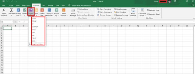
On the menu, you click formulas, next after the page layout tab.
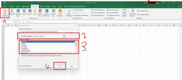
On the ribbon, you have two options.
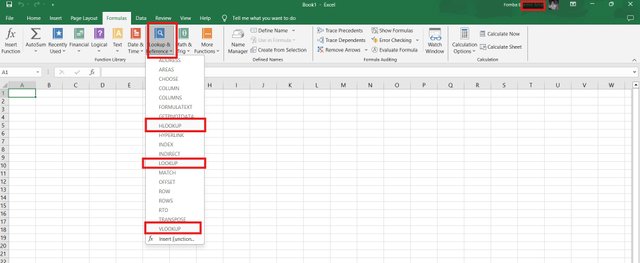
Click Insert functions, a longer process, or click Lookup & references.
By clicking Insert functions, a new tab will pop up. You used the drop-down to look for the Lookup function. Move down to select your desired lookup function and click okay.
Clicking the lookup & reference is more direct, as lookup functions are listed waiting to be selected.
Logical Functions
Logical Functions are conditional operations amid getting a Boolean data type result. The result is in two ways, either true or false. Some of the conditional statements in logical functions are IF, AND, OR, NOT, SWITCH, etc.
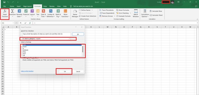
Launch the Microsoft Excel package
On the menu, you click formulas, next after the page layout tab.
Click Insert functions, a longer process, or click Lookup & references.
Write the IF Function formula to calculate the total, average score, and grade of students given in the table below.
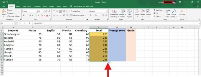
To get the total scores for all subjects, we will be making use of a simple SUM function. I have created a new column Total. Click in the first cell, to apply the function.
=SUM(B2:E2)
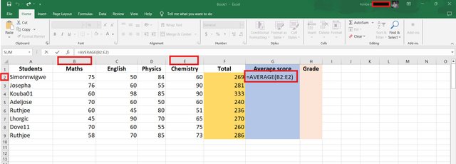
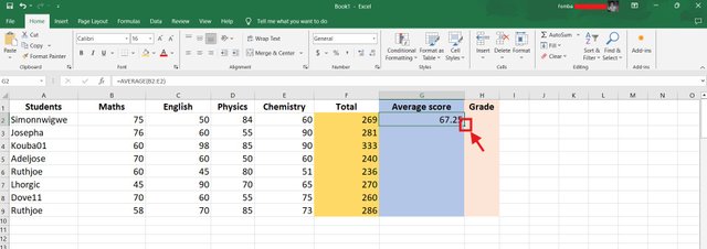
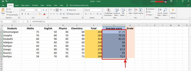
To calculate the average, we use the simple AVERAGE function. The steps are not different from that of the SUM.
=AVERAGE(B2:E2)
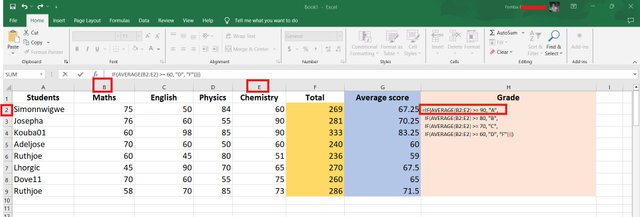
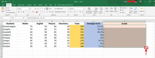
Calculating the grade required us to check if the value is true or false to give a specific grade. For this reason, a logical function is needed for me to be able to achieve a more efficient and accurate grade for each student. So we will make use of logical operators like >, <, =, >=, <=, or <> in our if statement based on the average score of each student.
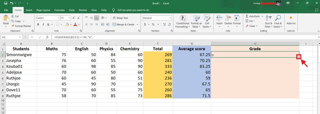
I will have more than one IF function separated by a comma, and each will check if the average score is greater than or equal to an assigned value. Then the grade will be outputted.
Method 1
=IF(AVERAGE(B2:E2) >= 90, "A",

IF(AVERAGE(B2:E2) >= 80, "B",

IF(AVERAGE(B2:E2) >= 70, "C",

IF(AVERAGE(B2:E2) >= 60, "D", "F"))))
Method 2
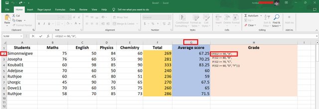
=IF(G2 >= 90, "A",

IF(G2 >= 80, "B",

IF(G2 >= 70, "C",

IF(G2 >= 60, "D", "F"))))
Both methods will give the same results; note method 1 makes use of the average function. Method 2 is making used of the results achieved in G2.
Briefly discuss four IF function Operators that you have learned and tell us their functions and when we are to use them.
IF Function formula is a logical function as mentioned above. It is used if the Function is to have results in a True state or a False state. This can only be achieved with logical operators in the If function.
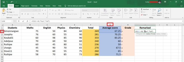
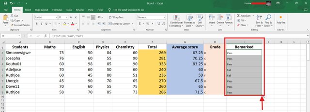
Greater Than (>): the greater than operator tells the function to check the values greater than another. In Excel, we can work with cells, or functions to compare their resulting values. When can we use it? We can use it to set a bar to validate the status of a student. I will use the average of the students in the table above to determine which student remarked.
=IF(G2 > 60, "Pass", "Fail")
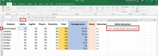
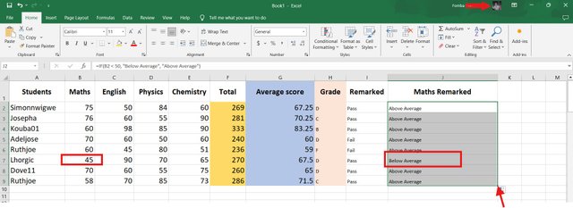
Less Than (<): The less-than operator is the opposite of the greater-than operator. The same principle applies to setting a threshold to differentiate a certain value from a particular target. 50 is our threshold to tell us which student had below average in maths.
=IF(B2 < 50, "Below Average", "Above Average")
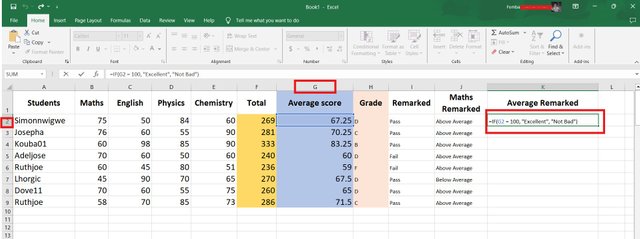
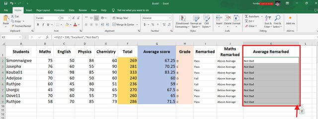
Equal To (=): The equal operation is used to check two values that are the same. This operator is used to check the exact values of a score.
=IF(G2 = 100, "Excellent", "Not Bad")
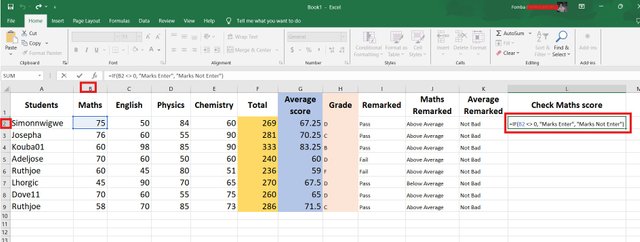
Not Equal To (<>): the not equal operator is used to check two values that do not match. This operator can be used to check errors on a sheet.
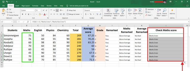
=IF(B2 <> 0, "Marks Enter", "Marks Not Enter")
Here, I was trying to the check the students whose marks were entered or who had a zero in Maths.
Based on the given data below: Create a pivot table that shows (see) total sales by product, by dragging the product to the Rows areas, Region to the Column area, and Sales to the Values area. Please we want to see the steps you take in adding your pivot table.
Since our available data is not huge, I will go ahead to demonstrate how to create a Pivot table on the same sheet.
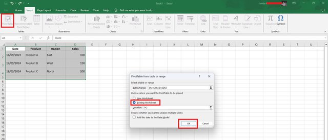
Click Insert and highlight all the cells containing the data.
Click Pivot table, and the new tab pops up
On the new tab, we can accurately input the data range needed. This in case we cannot highlight all cells necessary for the for the pivot table.
On this new tab, we have the possibility of creating our pivot on a new sheet. I mentioned I would be creating the pivot on the same sheet as the sheet holding the information.
The next requirement is the location on the same sheet, I input H2 and click Ok.
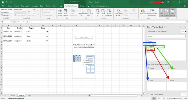
This time a sidebar is introduced holding data labels. to complete our task of creating the pivot table. On the sidebar, drag the label Products to the rows, drag Region to the column, and drag Sales to the value.
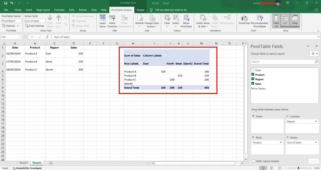
Our pivot table auto-generated using the date from the original table.
CONGRATULATIONS!!


