Calculation Study: Real functions. Part II

First of all I want to send a warm greeting to the communities of #steemstem y #utopian-io, for his special support for scientific, academic and intellectual articles.

In this opportunity I will give continuity to the series of the study of calculus: real functions. Part II In this case I will explain:

• The graph of a function.
• Classification of functions.
• Odd and even functions.

In the previous post: Study of Calculus: Real functions. Part I, addressed the following: function, domain and range of a function, graph of a function taking into account the geometrical criterion of the vertical line to know if an equation represents a real function or not. This publication will expand other fundamental concepts with which the part concerning real functions will be closed.

There are other types of evaluations that can be done with real functions, such as the growth and decrement criteria of a real function, asymptotes of a rational function, concavity criteria, extremes of a function (maximum points and minimum points). All this study can be done in this part but in an empirical way, since it is only with the criteria of the first and second derivative that the entire study can be completed, that is why this whole study will be fully explained in the corresponding publication of the derivative's applications.

With this publication, the study series of calculus will be closed: real functions. The continuity of the calculation study will remain open for the next publication, but this time it will be the series that deals with the limit of a function of a real variable.

Graph of a function

Remembering the geometrical criterion of the vertical line to be able to define if an equation is a function or not, we must know that this line must only cut the maximum graph in a single point, this means that for each element of the domain (real numbers in the X axis) only one element of the counter domain must correspond (real numbers on the Y axis). Once we are established in knowing that the equation is a function, whether we know it before or after it is plotted in the plane, it is where we can carry out the respective study of domain, rank and parity criteria.

There are two methodologies to my understanding to be able to make the graph of an equation by hand, that is without the help of computerized graphing, these are the following:

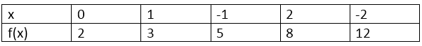
• If we do not know the basic behavior of the function we intend to graph: if we do not know what form the graph of a certain real function might have, the most suitable thing would be to construct a table of values where we can express the images of the function (f (x)) when x takes arbitrary values. Generally the arbitrary values of x that I advise to take are: 0,1, -1,2, -2. If by some circumstance with these values we still can not know what behavior the function takes, then we can expand them a little more, maybe it could be for x = {3, -3, 4, -4}. An example to get images can be:

Find the images needed for the function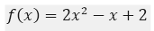

For this we will try giving arbitrary values ax of {0,1, -1,2, -2}, for those values of x when we introduce them in the equation of the function we will obtain a f (x) for each proposed arbitrary x, so the table would be as follows:

The problem presented here is due to the fact that for the proposed values of x, we have not obtained an image f (x) = 0, which implies that with those values of x we have not obtained the cut with the x axis. What is ideal for this case is to make f (x) = 0, which implies that 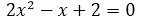, this represents a second degree equation equal to zero, therefore we must find the roots or values of x that annul the equation, as the equation is of the second degree, we will obtain two solutions, that is, a value of and . For this it is convenient to apply the equation of the resolvent:

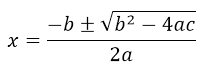; where for the equation:, where a=2; b=-1; c=2.

If we make the substitution of the values a, b and c, we would have:

= ⇒

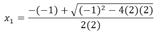In the result we can see that within the square root a negative value is remaining, and since the square root of a negative number does not give us a real result, it implies that both and there is no real solution, which means that the equation it has no real solution, and that the graph of the quadratic function does not have real cuts with the x-axis in the Cartesian system.

The importance of having met f (x) = 0 separately is that we conclude quickly that there is no value of x for which f (x) = 0, with this we limit the work of continuing to give arbitrary values ax in the table values.

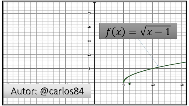
If we know the behavior of the graph of the function: if they give us the equation of a function, and we have the indication of knowing what the graphical behavior is, then it is advisable to apply the methodology of intersection with the coordinate axes Cartesian. The intersection with the coordinate axes is given by two types of useful solution points when plotting an equation, these are where the coordinate x or y is zero. Such points are called intersections with the axes because they are the points at which the graph intersects (intersects with) the x-axis or the y-axis. A point of type (a, 0) is an intersection with the x-axis of the graph of an equation if it is a solution point of it. To determine the intersections on the x-axis of a graph, f (x) = 0 is equated to then clear x from the resulting equation. Analogously, a point of the type (0, b) is an intersection with the y-axis of the graph of the equation that represents the function if it is a solution point of the same. To find the intersection with the y-axis, equal x to zero and clear the variable y = f (x) of the resulting equation.

It should be noted that this methodology of finding points intersection with the Cartesian axes, not only applies to real functions, but also for any type of equation that can be represented graphically in the two-dimensional plane (Cartesian plane).

To apply the methodology of points intersection with the Cartesian axes, we will take the following example:

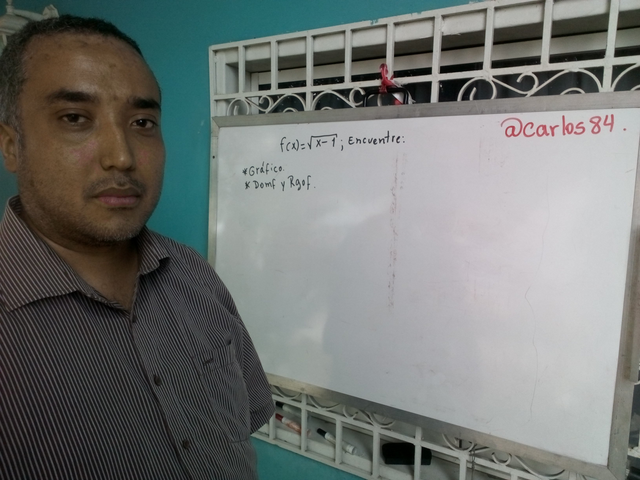
Find the points of intersection with the coordinate axes of the graph whose function is

Solution:

• To determine the intersections with the x axis, we make f (x) = 0; and we clear x.

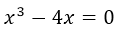⇒; as on the left side of equality we have x as a common element, so we take common factor x.

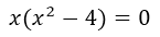⇒ ; the x that we have outside the parentheses as a common factor is our first solution of the third degree equation.

⇒

To get the remaining two solutions, we take the equation that is inside the parentheses and we equate it to zero and we clear the x.

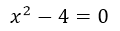
We already have the three solutions that represent the three cuts with the x axis, which would be: ; ;

These three solutions of the equation were to equal f (x) = 0, so the resulting points in the coordinate plane (x, y) are:
(0,0); (2.0); (-2.0)

To find the intersections with the y axis, we equal the x to zero.

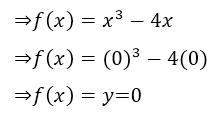
There are certain graphic peculiarities that have this cubic function that can not be covered with the criterion of intersections with the Cartesian axes, nor finding the images f (x) for arbitrary values of x, these particularities are those of being able to determine the maximum points and minimum of function 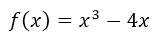, since to obtain these relative extremes, the first derivative criterion must be applied, and that is the reason for another publication.

Classification of functions

The modern notion known today of function is the result of the efforts of many mathematicians of the seventeenth and eighteenth centuries. Times that currently makes mathematicians like Leonhard Euler have to attribute a special mention to him because of the notation y = f (x). By the end of the eighteenth century, mathematicians and scientists had come to the conclusion that a large number of real-life phenomena could be represented by mathematical models, constructed from a collection of functions called elementary functions. These functions are divided into three categories:

1. Algebraic functions (polynomial, radical and rational).
2. Trigonometric functions.
3. Exponential and logarithmic functions.

In the present publication the functions will not be explained: trigonometric, inverse trigonometric, exponential and logarithmic, since the post will not be so extensive, I will treat them in a later publication where I will deal with their graphs, derivatives and integrals.

For this publication I will deal with the most known algebraic functions, which are the polynomial functions:

Where the positive integer n is the degree of the polynomial function. The constants are called coefficients, being the dominant coefficient and he constant term. In general, polynomial functions in their first degrees are usually expressed as follows:

Grade zero:

Grade one: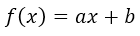

Grade two: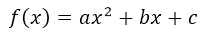

Grade three:

Test criteria for even and odd functions

• The function y = f (x) is even if f (-x) = f (x)
• The function y = f (x) is odd if f (-x) = -f (x)

To test this criterion, and thus be able to determine if a function is even or odd, we have the following example: Determine if It's even or odd, or neither.

Solution:

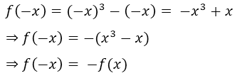
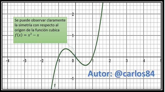
Since it complies with the second criterion, we can say that the function is odd and at the same time we can say that it is symmetric with respect to the origin.

In order to visualize the graph and see the symmetry with respect to the origin, we will use the software geogebra 5.0 to graph the function 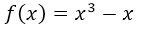. El gráfico se exportará del software como imagen para ser editado en Microsoft PowerPoint:

Conclusion and considerations

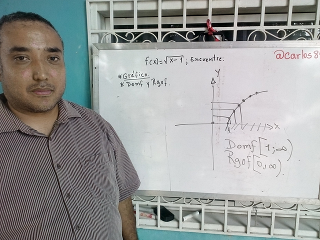
Once the optimal learning level of the real functions has been reached, we must be able to graph a function of the algebraic type, either polynomial or radical. Subsequently, we must also be able to carry out the respective study such as being able to determine the domain and range of the function, study the parity and the criteria of symmetry.

When it is already possible to explain the applications that the derivative has with the drawing of curves, we will be able to define all the parameters present when plotting a function, however the principles given in the first and second part of the series "Study of the Calculation referring to the real functions sow the solid bases for the plotting of the most known algebraic functions.