How to draw an evolutionary tree: UPGMA
In my first post, I explained how to read a phylogenetic tree, a tree depicting the relationship between different taxa, i.e. groups of organisms. In my second post, I explained what data forms the basis of such trees, and why molecular data are preferred over morphological (appearance-related) data. Now, the time has come to look into the process of constructing the trees, once we have our data.
Even with a relatively small number of taxa, the number of possible trees connecting them is huge. To find the most plausible tree, we need to make some assumptions and apply an appropriate algorithm. It may seem weird that several algorithms exist for calculating the "best" tree when, in reality, only one tree can be correct for any given dataset. Fortunately, the algorithms tend to agree quite well with each other. Some algorithms are fast, others are slower but make less drastic assumptions. With modern-day computers, even algorithms in the slow end of the spectrum can often be applied in a matter of seconds. Therefore, it's generally inadvisable to apply a fast, sloppy technique unless you have a good reason to assume that the underlying assumptions hold true. And yet, that's exactly the kind of technique I'm going to teach you in this post. Why? Because it's fast and one of the few that you can apply with pen and paper in a reasonable amount of time. Slightly more complicated techniques will follow in later posts.
I used to pronounce UPGMA letter by letter, but my wonderful statistics teacher always pronounced it like a real word ("up g'mah"), and I've adopted the habit. UPGMA stands for Unweighted Pair Group Method with Arithmetic Mean and is a lot easier than it sounds.
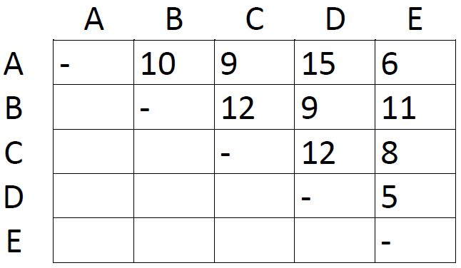
First off, we need a matrix listing the number of differences (e.g. base differences in homologous DNA sequences) between different taxa. Here's a mocked-up dataset with five taxa, labeled A-E:
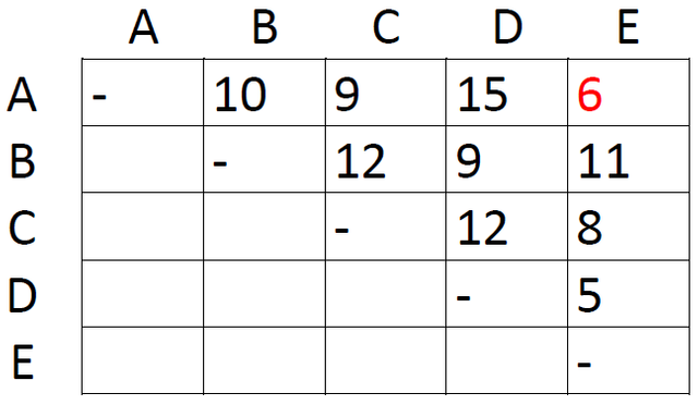
The first step is very simple. Just locate the shortest distance in the matrix:
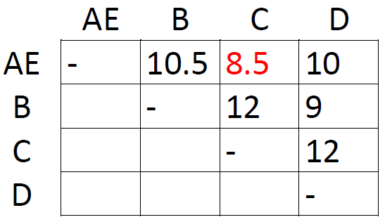
This is the distance between taxon A and taxon E. Since this is the shortest distance between any two taxa, we assume that A and E are each other's closest relative. We therefore group them together as AE and proceed to construct a new matrix with one row and one column less than the first one:
How did we obtain the new distances? By taking averages. For instance, the distance between A and B in the first matrix was 10, and the distance between B and E was 11. The distance from B to the new cluster AE is 10.5, the average of 10 and 11. This is where UPGMA makes a critical assumption, namely that the rate of evolution is constant throughout the tree. More complicated algorithms do not assume a constant rate of evolution, but for the sake of simplicity we accept it here. Distances that do not involve our newly formed cluster are not changed in the new matrix; the distance from C to D continues to be 12.
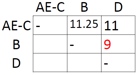
The shortest distance in the new matrix is the one connecting AE and C, so let's form the cluster AE-C and draw another matrix:
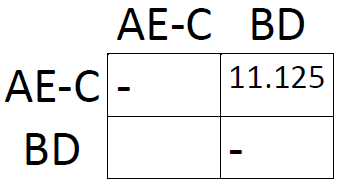
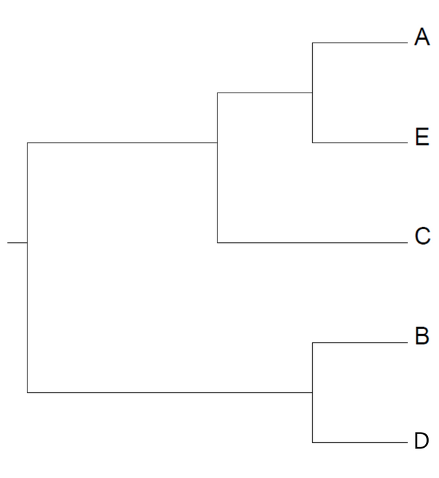
Same procedure as last time: take averages and find the smallest distance. This time, it's the one connecting B and D. This concludes our analysis:
Here's the tree:
Book reference
Marketa Zvelebil and Jeremy O. Baum (2008): "Understanding Bioinformatics"
Get free upvotes your post https://mysteemup.club