How to build a cat detector with a Raspberry Pi and a Pi Noir camera using Deep Learning - Part III

mragic (25)in #raspberrypi • 5 years ago (edited)

Part I is here:
https://steemit.com/raspberrypi/@mragic/how-to-build-a-cat-detector-with-a-raspberry-pi-and-a-pi-noir-camera-using-deep-learning-part-i
Part II:
https://steemit.com/raspberrypi/@mragic/how-to-build-a-cat-detector-with-a-raspberry-pi-and-a-pi-noir-camera-using-deep-learning-part-ii

Introduction

In this part III I will describe how the the images taken in can be used to train a deep neural network to distinguish images with cats against images without cats. This will need a lot of computing power, and if available a GPU (graphics card) with CUDA, and cannot be done reasonably on a raspberry pi. I use my Windows 10 notebook with a NVIDIA Geforce 1070 graphics card. In total I collected 14000 images with cats, and around 40000 images without cats. With this amount of data I can reasonably distinguish cats pictures from non-cat pictures with a probability of around 95%. The training of the neural network took around 36 hours.

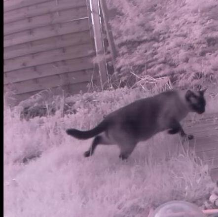
Example of a cat image, used to train the deep neural network

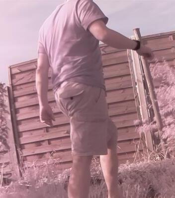
Example of a non-cat image used to train the deep neural network

Preparation of Software

You can get all the code here:

git clone https://github.com/magictimelapse/CatRecognition

First we will use anaconda as a python package manager to install all required python modules. You can download it from here:
https://www.anaconda.com/download/
I use the python 3.6 version.
Then open the anaconda shell from the start menu (called anaconda prompt). Create a anaconda environment with

conda create -n ai python=3.6

Press y to install all modules.
Activate this environment with

<condapath>/bin/activate ai

If you have GPU with CUDA feature (all modern NVIDIA GPUs have that), then install CUDA following this instruction:
https://www.tensorflow.org/install/gpu
for Windows or Linux, respectively.
Then install tensorflow. If you have a GPU use the module tensorflow-gpu, otherwise tensorflow:

conda install tensorflow-gpu

As deep learning framework, we will use the keras framework on top of tensorflow. Install it with:

conda install keras

For plotting of some graphs, we will use plotly. For image manipulation, we need pillow.

conda install plotly
conda install pillow

Preparation of the Data

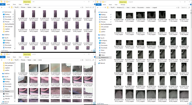
To train the deep neural network, we will need training data with label either cat or noCat assigned. We will thus split the cropped images in two folders, called cat and noCat. This can be done efficiently by copying all images to the windows computer to a folder called images. Create two folders cat and noCat, then copy from the images folder to either cat or noCat depending if there is a cat in the image or not. This can be done quite efficiently with all 3 folders open in the same desktop.

Yes, I did that for 14000 cats. I collected the images over around 2 months...

Finally, we need from both cat and noCat label around 10% of the images to test the deep neural network, and 90% of the images to train the network. I create two folders train and test, with each two folder cat and noCat, and copy each 10% of the images to the test folder and 90% to the train folder. Now we are ready to train our deep neural network!

Training of the Deep Neural Network

Recognizing and labeling of objects in images is a hot topic obviously, and huge advances where made in the last 5 years. There is yearly competition to compare labeling of thousands of categories, for example :
9: 'ostrich, Struthio camelus',
10: 'brambling, Fringilla montifringilla',
11: 'goldfinch, Carduelis carduelis',
12: 'house finch, linnet, Carpodacus mexicanus',
13: 'junco, snowbird',
14: 'indigo bunting, indigo finch, indigo bird, Passerina cyanea',
15: 'robin, American robin, Turdus migratorius'
See here: https://gist.github.com/yrevar/942d3a0ac09ec9e5eb3a for all categories.
It can also recognise different cats:
281: 'tabby, tabby cat',
282: 'tiger cat',
283: 'Persian cat',
284: 'Siamese cat, Siamese',
285: 'Egyptian cat',

Google's implementation of deep neural network is obviously quite good in this challenge (e.g. GoogleNet (aka inception v1)). So in a first trial, I just loaded the inception v3 model with the weights already trained with the imagenet data, which is conveniently already available in keras (see https://keras.io/applications/#inceptionv3). I realized though that it performs very poorly. Mostly because the images I took with the Pi Noir Camera are usually out of focus and the colors are obviously wrong. I also only want to distinguish cat from noCat, and don't care what kind of cat uses my garden as a toilet.

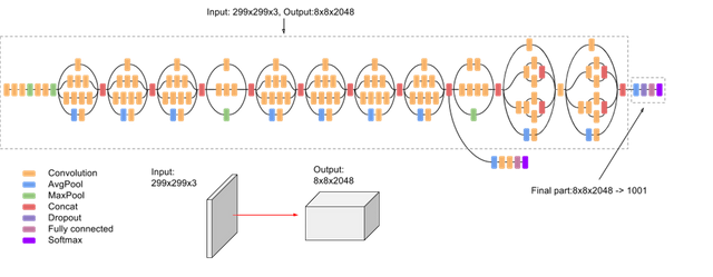
The inception v3 deep neural network, from: https://cloud.google.com/tpu/docs/inception-v3-advanced
The pretrained network can still be used, especially the first layers, as they are pretty general for image recognition tasks. They mostly discover image features like edges, or same color areas etc. We will use the pretrained inception v3 model, and replace the very last layer with a fully connected dense layer with two output categories. When training, we will leave all weights of the bottom layers unchanged and will only train the replaced layer with the two output categories "cat" and "noCat". This is called transfer learning and is used efficiently in different scenarios.
In above image, we thus will remove the final part 8x8x2048 -> 1001 categories and replace it with something that maps to 2 categories.
There are also other pretrained models you can try out, see here: https://keras.io/applications/
I tried all of them and found the performance of inception v3 the best. It seems to be best suited for transfer learning of out of focus images with wrong colors.

Running the Transfer Learning Training

You can download the transfer learning code from here:

git clone https://github.com/magictimelapse/CatRecognition

Some explanation of the code:

img_width, img_height = 299, 299
train_data_dir = "<set your directory with the training data here>"
validation_data_dir = "<set your diretory with the test data here>"

batch_size = 6
initial_epoch = 0
endepochs = 10

In train_data_dir and validation_data_dir set the training directory and the validation directory. batch_size is the number of images the neural network is optimised in one go. Set it larger to be faster, and smaller to be more precise. Initial_epoch and end_epoch is the number of epochs it will train (start to end). Set initial_epoch to 0, otherwise the program will load an existing pre trained neural network. One epoch is one iteration of the weight optimisation through all data. Run it first with a small number of epochs and check how long one epoch takes.

def add_last_layer(base_model, nb_classes = 2):
    x = base_model.output
    #x = Dropout(0.4)(x)
    x = Dense(16,activation="relu")(x)
    #x = Dropout(0.4)(x)
    predictions = Dense(nb_classes, activation='softmax')(x)
    model = Model(input=base_model.input, output=predictions)
    return model
def exchange_last_layers(base_model, nb_classes=2):
    x = base_model.output
    x= GlobalAveragePooling2D()(x)
    x = Dropout(0.4)(x)
    x = Dense(4,activation="relu")(x)
    x = Dropout(0.4)(x)
    predictions = Dense(nb_classes, activation='softmax')(x)
    model = Model(input=base_model.input, output=predictions)
    return model

These two functions do all the magic with replacing the last layer, respectively adding an additional layer to extend the deep neural network. It takes any base model (e.g. inception v3) and exchanges the top layer (or adds an additional layer respectively) with a densely connected network. Important is than the last dense layer with nb_classes the number of categories we want to distinguish. We choose 2 (cat vs noCat).

if initial_epoch > 0:
    refit = True
else:
    refit = False

if not refit:
    if model_name == 'inception_v3_1' or model_name == 'inception_v3_2'or model_name == "InceptionResNet_V2_0":
        if (K.image_dim_ordering() == 'th'):
            input_tensor = Input(shape=(3, 299, 299))
        else:
            input_tensor = Input(shape=(299, 299, 3))
        if model_name == 'inception_v3_1':
            base_model = InceptionV3(input_tensor=input_tensor, weights='imagenet',
                                 include_top=False)
            mymodel = exchange_last_layers(base_model)
        if model_name == 'inception_v3_2':
            base_model = InceptionV3(input_tensor=input_tensor, weights='imagenet',
                                 include_top=True)
            mymodel = add_last_layer(base_model)

        elif model_name == "InceptionResNet_V2_0":
            base_model = InceptionResNetV2(input_tensor=input_tensor, weights='imagenet',
                                     include_top=False)
            mymodel = exchange_last_layers(base_model)


        for layer in base_model.layers:
            layer.trainable = False
        mymodel.compile(optimizer='rmsprop',
                      loss='categorical_crossentropy',
                      metrics=['accuracy'])

We will not refit if the initial epoch is zero. This means that we will construct a new model from e.g. inception v3 and construct a new top layer, as described above. After training the model, we will save it as a hdf5 file, so that we can later refit it, for example when we have collected more cat images. We can then restart the fitting at the epoch we stopped in the last training session, by setting the corresponding initial_epoch higher up in the code.
The model 'inception_v3_1' will exchange the top layer with our custom dense layer. The model 'inception_v3_2' will add an additional layer. You can extend this block with your custom models, or with any model from here: https://keras.io/applications/
Finally we will set the layers of the base model to not trainable, and will only train our new layer. This model will still have 8206 trainable parameters, which is still a lot! However, compared to the already trained 21,802,784 parameters in the inception v3 model, this really reduces the number of parameters a lot.

train_datagen = ImageDataGenerator(
rescale = 1./255,
horizontal_flip = True,
fill_mode = "nearest",
zoom_range = 0.3,
width_shift_range = 0.3,
height_shift_range=0.3,
rotation_range=30)
train_generator = train_datagen.flow_from_directory(
train_data_dir,
target_size = (img_height, img_width),
batch_size = batch_size,
class_mode = "categorical")

Here we initialize the ImageDataGenerator. The idea is that we take the images, and create from them more training data by flipping the images, by zooming, shifhting and rotating the images a bit. This will make the training much more robust. We do the same with the validation data.

checkpoint = ModelCheckpoint(model_name+'.h5', monitor='val_acc', verbose=1, save_best_only=False, save_weights_only=False, mode='auto', period=1)

When fitting, we set a checkpoint after each iteration, where the model is saved in a hdf5 file. This helps to continue after a crash.

class_weights = {class_dictionary['cats']:0.85,class_dictionary['noCat']:0.15}
print(class_dictionary)
history= mymodel.fit_generator(
    train_generator,
    epochs = endepochs,
    initial_epoch =  initial_epoch,
    validation_data = validation_generator,
    class_weight=class_weights,
    steps_per_epoch=len(train_generator) ,
   validation_steps = len(validation_generator),
    callbacks=[checkpoint])

Here, the heavy lifting will be done. First we tell keras, that it should weight the cat category with a weight of 0.85 and the noCat category with 0.15, due to the fact that I have much more noCat data than cat data. The we start the fitting with the transformed images from above. You will see an output like:

__________________________________________________________________________________________________
activation_94 (Activation)      (None, 8, 8, 192)    0           batch_normalization_94[0][0]
__________________________________________________________________________________________________
mixed10 (Concatenate)           (None, 8, 8, 2048)   0           activation_86[0][0]
                                                                 mixed9_1[0][0]
                                                                 concatenate_2[0][0]
                                                                 activation_94[0][0]
__________________________________________________________________________________________________
global_average_pooling2d_1 (Glo (None, 2048)         0           mixed10[0][0]
__________________________________________________________________________________________________
dropout_1 (Dropout)             (None, 2048)         0           global_average_pooling2d_1[0][0]
__________________________________________________________________________________________________
dense_1 (Dense)                 (None, 4)            8196        dropout_1[0][0]
__________________________________________________________________________________________________
dropout_2 (Dropout)             (None, 4)            0           dense_1[0][0]
__________________________________________________________________________________________________
dense_2 (Dense)                 (None, 2)            10          dropout_2[0][0]
==================================================================================================
Total params: 21,810,990
Trainable params: 8,206
Non-trainable params: 21,802,784
__________________________________________________________________________________________________
None
Found 51165 images belonging to 2 classes.
Found 1049 images belonging to 2 classes.
{'cats': 0, 'noCat': 1}
Epoch 1/10
2052/8528 [======>.......................] - ETA: 19:48 - loss: 0.2060 - acc: 0.4366

The loss and acc values are important number. loss is the parameter that is optimized by the deep neural network in the fitting step. Here we use as loss function the categorical_crossentropy. The training will try to minimize this value by optimizing the weights in the neural network using back propagation. To learn more about backpropagation and deep neural networks, I can highly recommand Andrew Ng's courses on coursera:
https://www.coursera.org/learn/neural-networks-deep-learning
The value acc is a metrics the neural network calculates for each training step. It is defined as:
accuracy = number of correct predictions / total number of predictions
and is measure of how precise the neural network predicts the correct category.

The script will produce two plots in html files: history.html and history_accuracy.html. It will show the development of the loss function and the accuracy as a function of training epoch for training and validation data. They should become smaller with training epochs, and should be about the same for a training epoch for training and validation data. If they are not similar, we probably overtrain the network. You can try to increase the dropout factor, or reduce the number of dense nodes in the exchange_last_layer() function.

#cats #deeplearning #ai #keras