A Guide to Feynman Diagrams in the Many-Body Problem: Feynman Diagrams, or How to Solve the Many-body problems by means of Picture
Feynman diagrams constitute what might indeed be called ‘perturbation theory in comic-book form.’

Previously, we've discussed the basic definition of a many-body problem. We also introduced fictitious bodies - the quasi particles and collective excitations- to simplify the treatment of complex systems with thousands of bodies involve. In this chapter we're going to discuss the following topics:

(created using typora)
1.1 Propagators – the heroes of the many body problem
How can we calculate the properties of these fictitious particles – such as the effective mass or the lifetime?
The answer lies in the power of the quantum field theories quantity known as the propagators or Green’s function. Propagators are essentially a generalization of ordinary green’s function usually encountered in electrodynamics. Green’s functions comes in all sizes and shape – one particle, two particle, no particle, advanced, retarded, causal, zero temperature, finite temperature.
3 reasons why propagators are popular
- They yield in a direct way the most important properties of the system
- They have simple physical interpretation which appeals to the intuition
- They can be calculated that is highly systematic (integration) and ‘automatic’
The many-body state  can be described using positions of each particle which is a function of time
  . Fortunately, we don’t actually need the complete detailed description of the location of each particle in the system, but rather the average behaviour of one or two typical particles which are described using one-particle propagator and two-particle respectively.
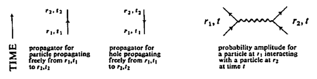
One-particle propagator
Given a particle at position r1 and t1, we will let it interact with other particles for a while (‘we let it propagate’), then the one-particle propagator is the probability of finding the particle at position r2 at time t2.
This propagator exposes the energies and the lifetime of quasi particles. In addition, momentum distribution, spin and particle density can also be calculated.
Two-particle propagator
With the same line of reasoning, allowing the particle to propagate for a while, the two-particle propagator is the probability amplitude for observing the particle at r1 (t1) in r2(t2) and r3(t4) at r4(t4). This propagator is useful for collective excitations, giving the energies, magnetic susceptibility, electrical conductivity, and a host of other non-equilibrium properties.
No-particle propagator
No-particle propagator is also called the ‘vacuum amplitude’. We put no particle into the system at time t1, and let the particles in the system interact with each other from t1 to t2, then ask for the probability amplitude that no particles emerge from the system at time t2.
This propagator is used to calculate the ground state energy and the grand partition function, from which all equilibrium properties of the system may be determined.
1.2 Calculating propagators by Feynman diagram
Two different methods for calculating the propagators
- Solve the chain of differential equations
- Expand the propagator in an infinite series and evaluate the series approximately
The latter can be achieved using the tools known as the Feynman Diagram.

To get the idea of Feynman diagram consider the diagram above, Propagation of Drunken Man. The man in the diagram leaves a party at point 1 and wants to go to his home at point 2. Along his path he can stop at one or more bars namely the Alice’s Bar (A), Bardot bar (B), Club Bar (C) , … etc.
The total probability  is given by the sum of the probabilities of each way,

This is an example of a ‘perturbation series’, with a bar as the ‘perturbations’ on the free propagation of the drunken man. Let’s introduce a ‘picture dictionary’ to associate each path to a particular picture.

Now, our ‘perturbation series’ can be drawn as:
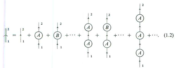
This series can be evaluated approximately by selecting the most important types of terms in it and summing them to infinity. This is referred to as the partial summation. For example, suppose the drunken man is in love with Alice, then we let P(A) have the large weights while the others P(X) are small.
We can then approximate equation 1.1 with majority of the interactions due to Alice as,
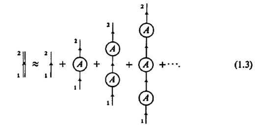
which can be translated in terms of probability functions:

We can simplify this equation by assuming that all intermediate interaction from r to s given by  are equal to the same number c. For instance,

We can write the series of 1.4 as,

The series in the bracket is the famous geometric summation, which yields,

Diagrammatically, this simplified version of the probability amplitude is given as,

For the rest of the section, we are going to use the partial summation method for strong interactions between particles in a many-body problems.
1.3 Propagator for single electron moving through a metal
Now, let’s consider a real physical system. Instead of a drunken man interacting with various bars, we will look at electrons interacting with various ions in a metal.
A metal consists of a positively charged ions arranged in a regular lattice or a lattice with irregularities due to some impurity.

The single particle propagator for this system is the quantum probability amplitude for all the possible ways the electron can propagate from point r1 in the crystal at t1 to point r2 at time t2, interacting with various ions along the way.
These are the possible path of the electron as it propagates to r2 from r1:
- Freely without interaction : 1-2
- Freely from r1 to ion in rA then to point r2: 1-A-2
- From 1 to ion B, interaction at B, then from B to 2: 1-B-2
- 1-A-A-2
- 1-A-B-2
etc.
This partial summation can also be visually represented by,
From the resulting propagator we obtain immediately the energy of the electron moving in the field of the ions.
1.4 Single-particle propagator for system of many interacting particles

Second-order Process
The figure shown above depicts a possible interaction with another particle. The first (a) is a free propagation without interaction. The event in (b) depicts a ‘second-order’ propagation process (a process with two interactions). Note, however, that these interactions are not real but rather ‘virtual’ or ‘quasi physical’. In reality, the figure is just a mathematical expression.
Sequence of events requires time, to do this, let us imagine that time increases in the upward-going direction:
(Note: hole is drawn as a particle moving backward in time, we'll encounter this particle in the future chapters).
The probability amplitude for the above sequence of events can be represented by the diagram.

This diagram:

is called the ‘self-energy‘ part because it shows the particle interacting with itself via the particle-hole pair it created in the many-body medium.
First-Order Process
Another sequence of events which can occur involves only the one interaction, also known as ‘first-order’ process.

The events sequence shown above involves a quick-change act in which the incoming electron at point r interacts with another electron at point r’ and changes place with it.
In diagram it is presented as,

The diagrams showing the sequence of events are called the Feynman diagrams after its inventor Richard Feynman. In his Nobel prize-winning work on quantum electrodynamics, he employed these diagrams. Nowadays, they are used extensively in elementary particle physics.
We’ve shown two possible even sequence already and in fact there is more possible sequence of events. The total single particle propagator is the sum of the amplitudes for all possible ways the particle can propagate through the system.
Thus we find,

This diagrams show all the configurations as it churns through the many-body system. At initial time, t0, various situations may exist: we have the bare particle (a), there may be two particles plus one hole created by the second-order process (c) or three particles plus two holes (d) etc.

Just like the drunken man, we can calculate the partial sum in this case in which we focus on a sequence of events that are more important. For instance, we can focus on the open oyster parts, since they constitute a geometric series form:

For the electron gas, this is the ‘Hartree-Fock’ approximation.
We can include ‘ring’ diagrams in the sum, in which the self-energy parts are composed of rings of particle-hole pair bubbles (these are the most important in a high-density electron gas):

This sum can be carried out and yields the so-called ‘random phase approximation’ or ‘RPA’ which is extremely useful in analysing the properties of metals.
Summary:
Note that the most important thing in a partial summation is the structure or topology of the diagrams, how various lines are connected to each other. This diagram topology is the key to the quantum field theoretical method in the many-body problem.
1.5 The two-particle propagator and the particle-hole propagator
For the two-particle propagator, it is simply the sum over the probability amplitude for all the ways two particles can enter the system, interact with each other and with the particles in the system, then emerge again.
The diagram even sequence is,

A partial sum over all the ‘ladder’ diagrams are:

‘Ladder approximation’ is useful in nuclear matter, and low-density systems.
Plasmons
The particle-hole propagator can be used to determine the energy and lifetime of collective excitations. For plasmons, its diagram is given as:

1.6 The no-particle propagator (‘vacuum amplitude’)
The no-particle propagator or ‘vacuum amplitude’ allows us to determine the many-body system ground state energy. This propagator is the sum of amplitudes for all the ways the system can begin at time t1 with no extra or lifted-out particles, or holes in it (this is the undisturbed or ‘Fermi vacuum’ state), have its particles interact with each other, and wind up at t2 with no extra or lifted-out particles, or holes.
The vacuum amplitude is represented by the following diagram:

In which (b) is a first-order process where two particles change places with each other as shown in the following diagram.

The vacuum amplitude series gives us a vivid picture of the ground state of the many-body system as a sort of ‘virtual witches’ brew, constantly seething, with particles and holes boiling up, bubbling, and colliding.
Appealing Features of Feynman Diagram
- They show directly the physical meaning of the perturbation term they represent
- They reveal at a glance the structure of very complicated approximations by showing which sets of diagrams have been summed over
Feynman diagrams constitute what might indeed be called ‘perturbation theory in comic-book form.’
Disclaimer: this is a summary of chapter 1 from the book A Guide to Feynman Diagrams: by Richard D. Mattuck, the content apart from rephrasing is identical, most of the equations are screenshots of the book and the same examples are treated.

