Time-Independent Schrodinger Equation and Hermitian Operators
Disclaimer: I lay no claim to the originality of the basic ideas expounded here. Its distinctness lies more in its scope and in the detail of its exposition.
Okay, the previous section's was littered with a little math. Now comes more math.
Stationary states and the time-independent Schrodinger equation
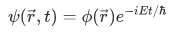
Previously, we have derived the Schrodinger equation by transforming the classical energy into operators. Today, we will specialize to the case when the particle is in a state with definite energy E. From the first section, we've derived that following form,
where  specifies the space-dependent part of the function. Let's take the absolute modulus of this wave function to obtain the probability amplitude,
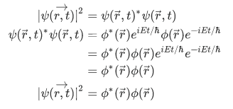
It is obvious that our time amplitude, 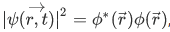 is time independent, such a state is called stationary state.
Now, lets substitute the time-dependent solution we have to the Schrodinger equation,
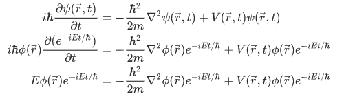
after some cancellation of the factor  , we obtain,
But note that our potential is still a time dependent. It turns out that for a definite energy to be attained, our potential-energy function must be time independent. We can replace 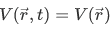 . And we have,
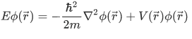
This equation is the time-independent Schrodinger equation, and is an eigenvalue equation of the form
with
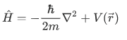
This operator
 is known as the Hamiltonian operator.
Eigenvalue spectra and the results of measurements
Recall the following equation of the previous sections,
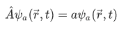
The set of all possible eigenvalues a of an operator  is called the spectrum of the operator . And for any physically realizable measurement of the observable A, it will always yield a value belonging to this spectrum.
For this eigenvalue problem there are two cases that we should consider.
Case 1
The wave function  describing the state of the particle is an eigenfunction
  of
of  , that is,
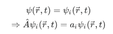
Then the result of measuring A will certainly be 
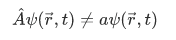
Case 2
The wavefunction  describing the state of the particle is not eigenfunction of
  that is, the action of
  on
on  gives a function that is not simply a scaled version of .
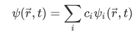
But since the eigenfunctions  of
of  form a complete set, in the sense that any normalized function can be expanded in terms of them, we may write
  as such an expansion:
Then we have,
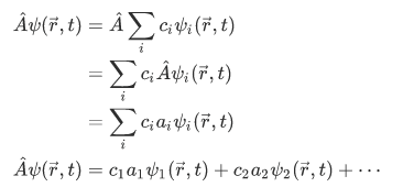
For this case, the result of measuring A yields the result  with probability
Hermitian Operators
One might wonder if all observable have an equivalent operators. It turns out there is a condition for an observable to have an equivalent operator, that is, the physical observable operator must be Hermitian.
Consider the textbook definition of a Hermitian operator.
Definition An operator  is said to be hermitian if for any pair of normalizable wave function
  and
and  , the relation
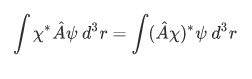
always hold.
Two important properties of Hermitian operators:
1. The eigenvalues of Hermitian operators are always real.
Proof:
Choose a  that are of the same with the wave function
  of the operator, with corresponding eigenvalue
  that is, we let
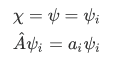
Using our definition of hermitian, we have
that is,
 , or, in other words, the eigenvalue is real.
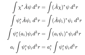
2. Hermitian operators corresponding to different eigenvalues has eigenfunctions that are orthogonal to each other
Proof:
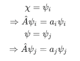
Now, choose  to be different eigenfunctions of
  with the corresponding eigenvalues,
Again, using the definition of hermitian,
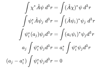
Utilizing the first fact that  , we have
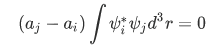
since
 we must have:
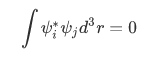
We say that
 is orthogonal with the wave function
  .
.
Remember this two facts about Hermitian operators they will come handy in almost all problems in quantum mechanics. For the moment, we will use the idea of orthogonality to prove an inequality:
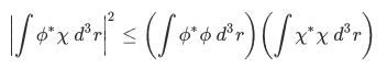
(we will use this to prove the general uncertainty relation in future sections). To prove this inequality, let's divide it into two case.
Case 1
The case where the function  corresponds to the equality.
Case 2
For the case where  we will express it as linear combination in terms of each other.
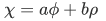
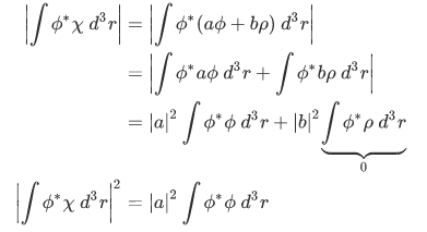
If the function
 is not only proportional to
  but also a part proportional to a normalized function
  orthogonal to , with
  (where
  ), we have:
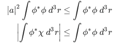
but then , so we have,
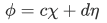
Similarly, expressing
 in terms of
  with the function
  orthogonal to
  and with both function normalized to unity so that
 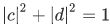 , we have
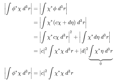
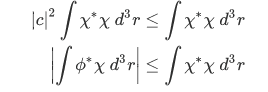
but then
 so we have,
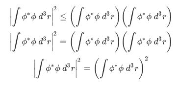
Multiplying the results of 1 and 2, we have,
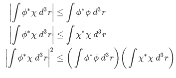
Therefore, we obtain the inequality. Q.E.D.
This post has received a 12.50% upvote from @lovejuice thanks to @pauldirac. They love you, so does Aggroed. Please be sure to vote for Witnesses at https://steemit.com/~witnesses.