5-19 Iris flowers dataset 적용 Linear Discriminant Analysis II: LDA Graph

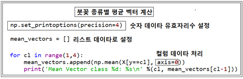
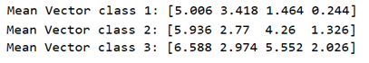
LDA 첫 단계로서 3가지 붓꽃 데이터 샘플 종류별 즉 class 라벨별로 평균 벡터를 구하자.

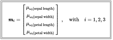
평균 벡터는 리스트형으로서 mean_vectors 라는 변수 명을 부여하자.

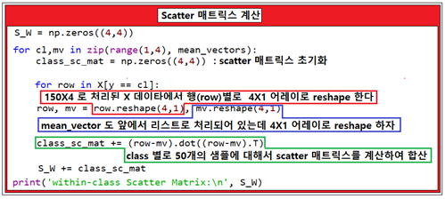
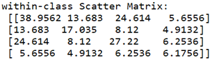
두 번째 단계에서는 3가지 붓꽃 종류 각각 별로 scatter 매트릭스에 해당하는 within-class scatter 매트릭스를 계산하자.

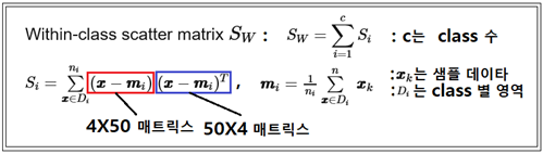
각 클래스 별 50개의 붓꽃 샘플 데이터들은 각각 꽃받침과 꽃잎의 길이와 폭 즉 4개의 독립적인 데이터로 이루어져 있다. 즉 4X50 매트릭스와 50X4 매트릭스를 곱하면 4X4 매트릭스가 얻어진다.

앞의 수치예제에서는 class 별 scatter 매트릭스를 계산 후 샘플수로 나누었는데 여기서는 샘플수로 나누지 않았다는 점에 유의하자. 샘플수를 고려하여 나누어 주는 경우는 scatter라고 하지 않고 covariance 라고 하며 unbias 된 경우 반드시 class 별로 (샘플수-1) 로 나누어 주어야 한다. 붓꽃 데이터 베이스는 3가지 class의 부분집합으로 이루어져 있으므로 각 class 별 (샘플수-1) 처리를 해 주어야 이를 사용하여 계산한 분산 값과 전체 150개로 이루어진 샘플(population)에서 직접 계산한 분산 값이 같아지게 된다. 즉 covariance 값을 계산하여 처리하려면 다음과 같이 (샘플수-1) 만큼 곱하도록 한다.

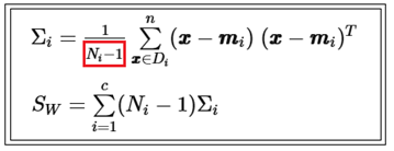
Within-class scatter 매트릭스에서는 covariance 가 아닌 scatter 방식으로 계산하기 때문에 Between-class scatter 매트릭스에서는 covariance가 아니므로 (샘플수-1)이 아닌 샘플수 자체를 곱하도록 한다.

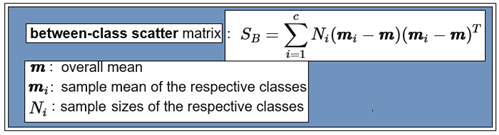
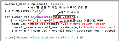
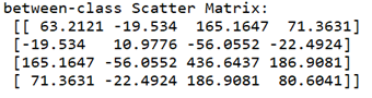
전체 평균값 및 각 class 샘플 별 갯수를 계산한다. 아울러 각 4X1 샘플 별 평균에서 전체 평균을 뺀 후 역행렬과 곱하여 누적한다.

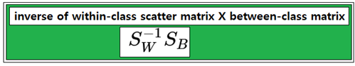
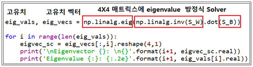
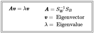
Within –class scatter 매트릭스의 역행렬과 between-class scatter 행렬을 곱한 후 eigenvalue 문제로 정식화 하여 풀도록 한다.

Fisher 의 Linear Discriminant 조건은 다음과 같다.

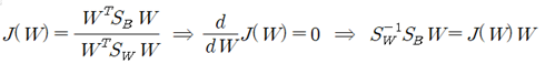
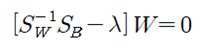
이 식에서 특정한 W 값에서 위 등식을 만족하는 조건을 적용하여 eigenvalue 방정식을 유도하자.

numpy 와 lapack 라이브러리를 사용하여 풀어서 eigenvalue 와 eigenvector를 계산하자.

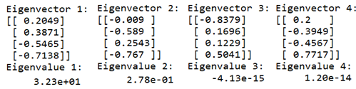
4개의 eigenvalue 값이 얻어지는데 그 값들이 가지게 되는 정보 또는 의미를 파악해 보자.

eigenvalue 와 eigenvector는 선형변환 결과에 대한 정보를 제공하는데 특히 eigenvector는 변환의 방향을 지시하며 eigenvalue는 그 크기가 1.0 인 eigenvector의 축척으로 사용이 가능하다.

계산된 eigenvalue와 eigenvector를 대입하여 만족 여부를 체크해 본다.

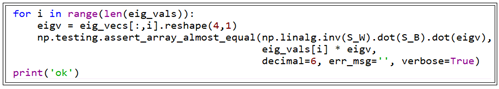
대입해서 처리된 결과가 성공적이면 ‘ok’를 출력한다.
이미 계산된 eigenvalue 중에서 어느 것이 가장 유용한 정보를 제공할지 알아보자. 일단 크기순으로 처리하도록 한다. 물론 3번과 4번의 eigenvalue 값은 0.0 이므로 고려 대상에서 제외시키자.

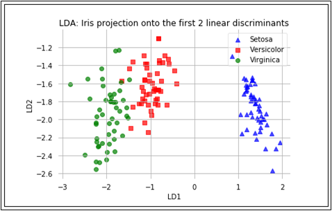
LDA 이론에서 주어진 데이터를 한 차원 낮은 공간으로 투영함으로 인해 class 별 Classification 이 쉬워질 수 있다는 점을 지적하였다. 여기서는 150개로 이루어진 즉 150X4 크기의 X 데이터와 4X4 로 계산된 eigenvector W 중에서 eigenvalue 가 실질적으로 0.0 인 2개의 컬럼을 배제한 4X2 eigenvector W를 곱하여 선형변환을 하도록 한다. 선형 변환의 결과는 운 좋게도 150X2 매트릭스로 얻어질 것이다. 즉 평면상에 작도가 가능하다.

#Iris_lda_matrix_01.py
import pandas as pd

s1 = 'sepal length cm'
s2 = 'sepal width cm'
s3 = 'petal length cm'
s4 = 'petal width cm'

feature_dict = {i:label for i,label in zip(range(4),( s1, s2, s3, s4))}

df = pd.io.parsers.read_csv(filepath_or_buffer=
'https://archive.ics.uci.edu/ml/machine-learning-databases/iris/iris.data',
header=None,sep=',',)
df.columns = [l for i,l in sorted(feature_dict.items())] + ['class label']
df.dropna(how="all", inplace=True) # to drop the empty line at file-end

df.tail()

from sklearn.preprocessing import LabelEncoder

X=df[[ s1, s2, s3, s4]].values
y = df['class label'].values

enc = LabelEncoder()
label_encoder = enc.fit(y)
y = label_encoder.transform(y) + 1

label_dict = {1: 'Setosa', 2: 'Versicolor', 3:'Virginica'}

from matplotlib import pyplot as plt
import numpy as np
import math

fig, axes = plt.subplots(nrows=2, ncols=2, figsize=(12,6))

for ax,cnt in zip(axes.ravel(), range(4)):

# set bin sizes
min_b = math.floor(np.min(X[:,cnt]))
max_b = math.ceil(np.max(X[:,cnt]))
bins = np.linspace(min_b, max_b, 25)

# plottling the histograms
for lab,col in zip(range(1,4), ('blue', 'red', 'green')):
    ax.hist(X[y==lab, cnt],color=col,
               label='class %s' %label_dict[lab],
               bins=bins,alpha=0.7,)
ylims = ax.get_ylim()

# plot annotation
leg = ax.legend(loc='upper right', fancybox=True, fontsize=8)
leg.get_frame().set_alpha(0.5)
ax.set_ylim([0, max(ylims)+2])
ax.set_xlabel(feature_dict[cnt])
ax.set_title('Iris histogram #%s' %str(cnt+1))

# hide axis ticks
ax.tick_params(axis="both", which="both", bottom="off", top="off",  
        labelbottom="on", left="off", right="off", labelleft="on")

# remove axis spines
ax.spines["top"].set_visible(False)  
ax.spines["right"].set_visible(False)
ax.spines["bottom"].set_visible(False)
ax.spines["left"].set_visible(False)    

axes[0][0].set_ylabel('count')
axes[1][0].set_ylabel('count')

fig.tight_layout()

plt.show()

np.set_printoptions(precision=4)

mean_vectors = []
for cl in range(1,4):
mean_vectors.append(np.mean(X[y==cl], axis=0))
print('Mean Vector class %d: %s\n' %(cl, mean_vectors[cl-1]))

S_W = np.zeros((4,4))
for cl,mv in zip(range(1,4), mean_vectors):
class_sc_mat = np.zeros((4,4)) # scatter matrix for every class
for row in X[y == cl]:
row, mv = row.reshape(4,1), mv.reshape(4,1) # make column vectors
class_sc_mat += (row-mv).dot((row-mv).T)
S_W += class_sc_mat # sum class scatter matrices
print('within-class Scatter Matrix:\n', S_W)

overall_mean = np.mean(X, axis=0)

S_B = np.zeros((4,4))
for i,mean_vec in enumerate(mean_vectors):
n = X[y==i+1,:].shape[0]
mean_vec = mean_vec.reshape(4,1) # make column vector
overall_mean = overall_mean.reshape(4,1) # make column vector
S_B += n * (mean_vec - overall_mean).dot((mean_vec - overall_mean).T)

print('between-class Scatter Matrix:\n', S_B)

eig_vals, eig_vecs = np.linalg.eig(np.linalg.inv(S_W).dot(S_B))

for i in range(len(eig_vals)):
eigvec_sc = eig_vecs[:,i].reshape(4,1)
print('\nEigenvector {}: \n{}'.format(i+1, eigvec_sc.real))
print('Eigenvalue {:}: {:.2e}'.format(i+1, eig_vals[i].real))

for i in range(len(eig_vals)):
eigv = eig_vecs[:,i].reshape(4,1)
np.testing.assert_array_almost_equal(np.linalg.inv(S_W).dot(S_B).dot(eigv),
eig_vals[i] * eigv,
decimal=6, err_msg='', verbose=True)
print('Eigenvectors:\n')
print(eig_vecs)
print('ok')

#Make a list of (eigenvalue, eigenvector) tuples
eig_pairs = [(np.abs(eig_vals[i]), eig_vecs[:,i]) for i in range(len(eig_vals))]

#Sort the (eigenvalue, eigenvector) tuples from high to low
eig_pairs = sorted(eig_pairs, key=lambda k: k[0], reverse=True)

#Visually confirm that the list is correctly sorted by decreasing eigenvalues

print('Eigenvalues in decreasing order:\n')
for i in eig_pairs:
print(i[0])

#magnitude comparison
print('Variance explained:\n')
eigv_sum = sum(eig_vals)
for i,j in enumerate(eig_pairs):
print('eigenvalue {0:}: {1:.2%}'.format(i+1, (j[0]/eigv_sum).real))

W = np.hstack((eig_pairs[0][1].reshape(4,1), eig_pairs[1][1].reshape(4,1)))
print('Matrix W:\n', W.real)

X_lda = X.dot(W)
assert X_lda.shape == (150,2), "The matrix is not 150x2 dimensional."
print(X_lda)

def plot_step_lda():

ax = plt.subplot(111)
for label,marker,color in zip(
    range(1,4),('^', 's', 'o'),('blue', 'red', 'green')):

    plt.scatter(x=X_lda[:,0].real[y == label],
            y=X_lda[:,1].real[y == label],
            marker=marker,
            color=color,
            alpha=0.7,
            label=label_dict[label]
            )

plt.xlabel('LD1')
plt.ylabel('LD2')

leg = plt.legend(loc='upper right', fancybox=True)
leg.get_frame().set_alpha(0.5)
plt.title('LDA: Iris projection onto the first 2 linear discriminants')

# hide axis ticks
plt.tick_params(axis="both", which="both", bottom="off", top="off",  
        labelbottom="on", left="off", right="off", labelleft="on")

# remove axis spines
ax.spines["top"].set_visible(False)  
ax.spines["right"].set_visible(False)
ax.spines["bottom"].set_visible(False)
ax.spines["left"].set_visible(False)    

plt.grid()
plt.tight_layout
plt.show()

plot_step_lda()