[머신러닝] XOR 문제 해결하기 Part.2
XOR 문제를 풀지 못해 머신러닝 개발이 늦어졌다가, backpropgation을 통해 풀어낼 수 있다는 사실 알아냈다. 이제는 TensorFlow로 직접 구현해보자.
XOR Data set
import numpy as np
import tensorflow as tf
먼저 그동안 학습해왔던 방식 그대로 XOR 문제를 풀어보자.
x_data = np.array([[0, 0], [0, 1], [1, 0], [1, 1]], dtype = np.float32)
y_data = np.array([[0], [1], [1], [0]], dtype = np.float32)

X = tf.placeholder(tf.float32)
Y = tf.placeholder(tf.float32)
W = tf.Variable(tf.random_normal([2, 1]), name = 'weight')
b = tf.Variable(tf.random_normal([1]), name = 'bias')

# Hypothesis using Sigmoid : tf.div(1., 1 + tf.exp(tf.matmul))
hypothesis = tf.sigmoid(tf.matmul(X, W) + b)

# cost/loss function
cost = -tf.reduce_mean(Y * tf.log(hypothesis) + (1 - Y) * tf.log(1 - hypothesis))
train = tf.train.GradientDescentOptimizer(learning_rate=0.1).minimize(cost)

# Accuracy computation
# True if hypothsis > 0.5 else False
predicted = tf.cast(hypothesis > 0.5, dtype = tf.float32)
accuracy = tf.reduce_mean(tf.cast(tf.equal(predicted, Y), dtype=tf.float32))

# Launch graph
with tf.Session() as sess:
    # Initialize TensorFlow Variables
    sess.run(tf.global_variables_initializer())

    for step in range(10001):
        sess.run(train, feed_dict={X: x_data, Y: y_data})
        if step % 1000 == 0:
            print(step, sess.run(cost, feed_dict={X: x_data, Y: y_data}), sess.run(W))

    # Accuracy report
    h, c, a = sess.run([hypothesis, predicted, accuracy], feed_dict={X: x_data, Y: y_data})
    print('Hypothsis : ', h, "Correct : ", c, "Accuracy : ", a)
그동안 우리가 해왔던 방식 그대로 sigmoid를 사용해 가설을 세우고 학습을 진행했다. chain-rule을 사용하지 않고 W와 b 값을 한 번에 예측했다. 결과를 보자.
0 0.76454574 [[0.72986054]
 [1.2056271 ]]
1000 0.6931765 [[0.02050375]
 [0.02141563]]
2000 0.6931472 [[0.00041052]
 [0.00041224]]
...
9000 0.6931472 [[1.3160042e-07]
 [1.3274089e-07]]
10000 0.6931472 [[1.3160042e-07]
 [1.3274089e-07]]
Hypothsis :  [[0.5]
 [0.5]
 [0.5]
 [0.5]] Correct :  [[0.]
 [0.]
 [0.]
 [0.]] Accuracy :  0.5
Accuracy가 50% 밖에 되지 않는다. 학습 데이터의 양이 극히 소수임에도 불구하고 거의 학습되지 않았다고 볼 수 있다. 동전을 던져서 한 쪽 면이 나올 확률과 같은 정확도다.
Neural Net for XOR
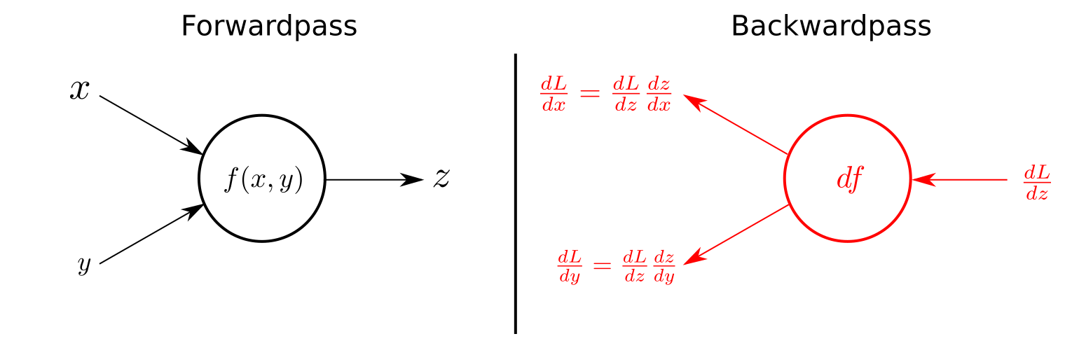
그렇다면 단계를 잘게 쪼개서 각 요소의 민감도를 분리해서 측정해보는 Chain-rule을 사용해보자. 이 그림을 떠올리면 된다.
x_data = np.array([[0, 0], [0, 1], [1, 0], [1, 1]], dtype = np.float32)
y_data = np.array([[0], [1], [1], [0]], dtype = np.float32)

X = tf.placeholder(tf.float32)
Y = tf.placeholder(tf.float32)

W1 = tf.Variable(tf.random_normal([2, 2]), name = 'weight1')
b1 = tf.Variable(tf.random_normal([2]), name = 'bias1')
layer1 = tf.sigmoid(tf.matmul(X, W1) + b1)

W2 = tf.Variable(tf.random_normal([2, 1]), name = 'weight2')
b2 = tf.Variable(tf.random_normal([1]), name = 'bias2')
hypothesis = tf.sigmoid(tf.matmul(layer1, W2) + b2)
W와 b가 두개로 늘어났다. 단 한 번에 가설을 만들어내지 않고, 두 단계에 걸쳐서 W1, b1, W2, b2를 계산해낸다.
# cost/loss function
cost = -tf.reduce_mean(Y * tf.log(hypothesis) + (1 - Y) * tf.log(1 - hypothesis))
train = tf.train.GradientDescentOptimizer(learning_rate=0.01).minimize(cost)

# Accuracy computation
# True if hypothsis > 0.5 else False
predicted = tf.cast(hypothesis > 0.5, dtype = tf.float32)
accuracy = tf.reduce_mean(tf.cast(tf.equal(predicted, Y), dtype=tf.float32))

# Launch graph
with tf.Session() as sess:
    # Initialize TensorFlow Variables
    sess.run(tf.global_variables_initializer())

    for step in range(10001):
        sess.run(train, feed_dict={X: x_data, Y: y_data})
        if step % 1000 == 0:
            print(step, sess.run(cost, feed_dict={X: x_data, Y: y_data}), sess.run(W))

    # Accuracy report
    h, c, a = sess.run([hypothesis, predicted, accuracy], feed_dict={X: x_data, Y: y_data})
    print('Hypothsis : ', h, "Correct : ", c, "Accuracy : ", a)
그리고 뒤의 코드는 기존의 코드와 동일하다. 예측 단계를 두 단계로 나눴을 때 어떤 결과가 나오는지 살펴보자.
0 0.8071356 [[-1.0126323 ]
 [-0.78457475]]
1000 0.7138937 [[-1.0126323 ]
 [-0.78457475]]
2000 0.69294065 [[-1.0126323 ]
 [-0.78457475]]
...
9000 0.5089611 [[-1.0126323 ]
 [-0.78457475]]
10000 0.45777205 [[-1.0126323 ]
 [-0.78457475]]
Hypothsis :  [[0.41157767]
 [0.6334697 ]
 [0.6129109 ]
 [0.2986155 ]] Correct :  [[0.]
 [1.]
 [1.]
 [0.]] Accuracy :  1.0
Accurary가 100%가 됐다. 단지 hypothesis를 도출해 내는 단계를 두 단계로 나눴을 뿐인데 정확도가 완벽해졌다. 우리가 세운 backpropagation 가설이 실제로 입증됐다는 의미다.
Wide NN for XOR
위의 데이터 셋은 극히 소량이기 때문에 실제 데이터의 양과는 괴리가 크다. 데이터의 양이 더 많아지고 복잡해질 수록 학습 알고리즘도 이를 수용할 수 있을만큼의 복잡도를 지녀야 한다. 이를 위해 두가지 방향성을 선택할 수 있다. Wide와 Deep. 넓거나 깊거나. 그리고 넓고 깊거나.
...
W1 = tf.Variable(tf.random_normal([2, 10]), name = 'weight1')
b1 = tf.Variable(tf.random_normal([10]), name = 'bias1')
layer1 = tf.sigmoid(tf.matmul(X, W1) + b1)

W2 = tf.Variable(tf.random_normal([10, 1]), name = 'weight2')
b2 = tf.Variable(tf.random_normal([1]), name = 'bias2')
hypothesis = tf.sigmoid(tf.matmul(layer1, W2) + b2)
...
이전 Neural Network에서는 W1의 형태가 [2, 2] 였다. 하지만 변수를 더 넓은 범위로 늘려서 측정함으로써 세세하게 쪼개어 민감도를 측정할 수 있다. 이제 W1의 형태는 [2, 10]이다. 더 넓어졌다.

Hypothsis :  [[0.33876547]
 [0.5671229 ]
 [0.6572764 ]
 [0.45574242]] Correct :  [[0.]
 [1.]
 [1.]
 [0.]] Accuracy :  1.0
역시나 정확도는 100%다. 워낙 작은 데이터 셋이기에 본 예시로는 변별력이 없지만 데이터가 커질 수록 학습 성능의 차이가 두드러진다.
Deep NN for XOR
마찬가지로 더 깊은 Neural Network도 가능하다. 이번에는 더 많은 chain을 연결하는 것이다. 물론 Deep과 Wide를 동시에 적용할 수 있다.
...
W1 = tf.Variable(tf.random_normal([2,10]), dtype=tf.float32)
b1 = tf.Variable(tf.random_normal([10]), dtype=tf.float32)
layer1 = tf.sigmoid(tf.matmul(X, W1) + b1)

W2 = tf.Variable(tf.random_normal([10,10]), dtype=tf.float32)
b2 = tf.Variable(tf.random_normal([10]), dtype=tf.float32)
layer2 = tf.sigmoid(tf.matmul(layer1, W2) + b2)

W3 = tf.Variable(tf.random_normal([10,10]), dtype=tf.float32)
b3 = tf.Variable(tf.random_normal([10]), dtype=tf.float32)
layer3 = tf.sigmoid(tf.matmul(layer2, W3) + b3)

W4 = tf.Variable(tf.random_normal([10,1]), dtype=tf.float32)
b4 = tf.Variable(tf.random_normal([1]), dtype=tf.float32)
hypothesis = tf.sigmoid(tf.matmul(layer1, W4) + b4)
...
Wide를 유지한채 더 많은 layer를 연결했다. 학습 단계가 더 깊어지면서 정확도를 개선하려는 의도다. Deep Learning이라는 개념을 상기해보자.
Hypothesis :  [[0.4165659 ]
 [0.5374485 ]
 [0.6033321 ]
 [0.46646127]] Correct :  [[0.]
 [1.]
 [1.]
 [0.]] Accuracy :  1.0
역시나 정확도는 100%다. 마찬가지로 데이터 셋이 많아지고 복잡해질수록 성능의 변별력이 드러날 것이다. 이제 우리는 수십년 전만 해도 풀 수 없다고 했던 XOR 문제를 풀 수 있게 되었다.
짱짱맨 호출에 출동했습니다!!