Quantitative Analysis of Digital Currency Market (2)

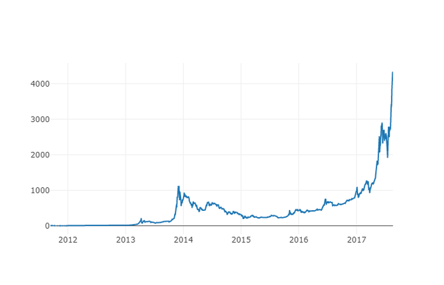
Next, we are going to make a simple table in order to verify the correctness of the data by visualization.

# Make a table of BTC prices
btc_trace = go.Scatter(x=btc_usd_price_kraken.index, y=btc_usd_price_kraken['Weighted Price'])
py.iplot([btc_trace])

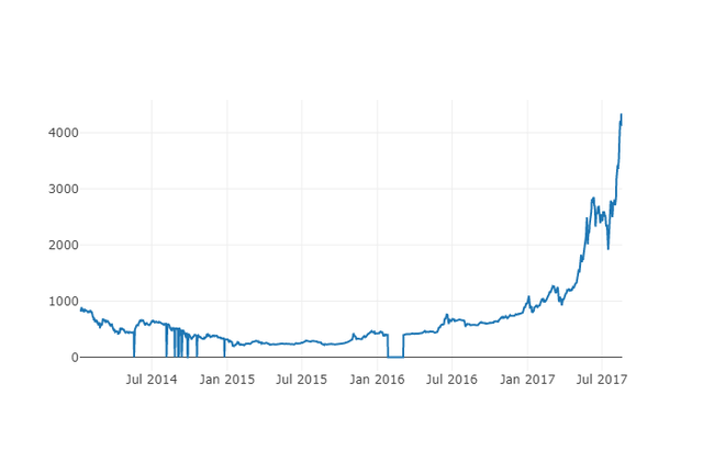
Here, we use Plotly to complete the visualization part. Compared with using some more mature Python data visualization libraries, such as Matplotlib, Plotly is a less common choice, but it is really a good choice, because it can call D3.js' fully interactive charts. These charts have beautiful default settings, which are easy to explore and very easy to embed into the web page.

Tips: The generated chart can be compared with the Bitcoin price chart of mainstream exchanges (such as the chart on OKX, Binance or Huobi) as a quick integrity check to confirm whether the downloaded data is generally consistent.

2.3 Obtain price data from mainstream Bitcoin exchanges

Careful readers may have noticed that there are missing data in the above data, especially at the end of 2014 and the beginning of 2016. Especially in Kraken Exchange, this kind of data loss is particularly obvious. We certainly do not hope that these missing data will affect the price analysis.

The characteristic of digital currency exchange is that the supply and demand relationship determines the currency price. Therefore, no transaction price can become the "mainstream price" of the market. In order to solve the problem and the data loss problem just mentioned (possibly due to technical power outages and data errors), we will download data from three mainstream Bitcoin exchanges in the world, and then calculate the average Bitcoin price.

Let's start by downloading the data of each exchange to the data frame composed of dictionary types.

# Download price data from COINBASE, BITSTAMP and ITBIT
exchanges = ['COINBASE','BITSTAMP','ITBIT']

exchange_data = {}

exchange_data['KRAKEN'] = btc_usd_price_kraken

for exchange in exchanges:
    exchange_code = 'BCHARTS/{}USD'.format(exchange)
    btc_exchange_df = get_quandl_data(exchange_code)
    exchange_data[exchange] = btc_exchange_df

2.4 Integrate all data into one data frame

Next, we will define a special function to merge the columns that are common to each data frame into a new data frame. Let's call it merge_dfs_on_column function.

def merge_dfs_on_column(dataframes, labels, col):
    '''Merge a single column of each dataframe into a new combined dataframe'''
    series_dict = {}
    for index in range(len(dataframes)):
        series_dict[labels[index]] = dataframes[index][col]
        
    return pd.DataFrame(series_dict)

Now, all data frames are integrated based on the "weighted price" column of each data set.

# Integrate all data frames
btc_usd_datasets = merge_dfs_on_column(list(exchange_data.values()), list(exchange_data.keys()), 'Weighted Price')

Finally, we use the "tail ()" method to view the last five rows of the merged data to ensure that the data is correct and complete.

btc_usd_datasets.tail()

The results are shown as:

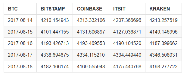
From the table above, we can see that these data are in line with our expectations, with roughly the same data range, but slightly different based on the delay or characteristics of each exchange.

2.5 Visualization process of price data

From the perspective of analysis logic, the next step is to compare these data through visualization. To do this, we need to define an auxiliary function first. By providing a single line command to use data to make a chart, we call it df_scatter function.

def df_scatter(df, title, seperate_y_axis=False, y_axis_label='', scale='linear', initial_hide=False):
    '''Generate a scatter plot of the entire dataframe'''
    label_arr = list(df)
    series_arr = list(map(lambda col: df[col], label_arr))
    
    layout = go.Layout(
        title=title,
        legend=dict(orientation="h"),
        xaxis=dict(type='date'),
        yaxis=dict(
            title=y_axis_label,
            showticklabels= not seperate_y_axis,
            type=scale
        )
    )
    
    y_axis_config = dict(
        overlaying='y',
        showticklabels=False,
        type=scale )
    
    visibility = 'visible'
    if initial_hide:
        visibility = 'legendonly'
        
    # Table tracking for each series
    trace_arr = []
    for index, series in enumerate(series_arr):
        trace = go.Scatter(
            x=series.index, 
            y=series, 
            name=label_arr[index],
            visible=visibility
        )
        
        # Add a separate axis to the series
        if seperate_y_axis:
            trace['yaxis'] = 'y{}'.format(index + 1)
            layout['yaxis{}'.format(index + 1)] = y_axis_config    
        trace_arr.append(trace)

    fig = go.Figure(data=trace_arr, layout=layout)
    py.iplot(fig)

For your easy understanding, this article will not discuss the logic principle of this auxiliary function too much. If you want to know more, please check the official documentation of Pandas and Plotly.

Now, we can create Bitcoin price data charts easily!

# Plot all BTC transaction prices
df_scatter(btc_usd_datasets, 'Bitcoin Price (USD) By Exchange')

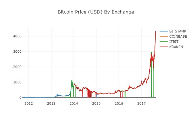
2.6 Clear and aggregate price data

As can be seen from the chart above, although the four series of data follow roughly the same path, there are still some irregular changes. We will try to eliminate these irregular changes.

In the period of 2012-2017, we know that the price of Bitcoin has never been equal to zero, so we remove all zero values in the data frame first.

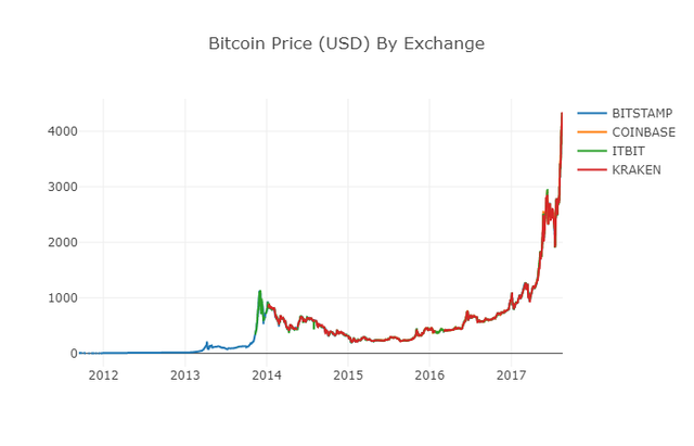
# Clear the "0" value
btc_usd_datasets.replace(0, np.nan, inplace=True)

After reconstructing the data frames, we can see a clearer chart with no missing data anymore.

# Plot the revised data frame
df_scatter(btc_usd_datasets, 'Bitcoin Price (USD) By Exchange')

We can calculate a new column now: the daily average Bitcoin price of all exchanges.

# Calculate the average BTC price as a new column
btc_usd_datasets['avg_btc_price_usd'] = btc_usd_datasets.mean(axis=1)

The new column is the price index of Bitcoin! Let's draw it again to check whether the data looks wrong.

# Plot the average BTC price
btc_trace = go.Scatter(x=btc_usd_datasets.index, y=btc_usd_datasets['avg_btc_price_usd'])
py.iplot([btc_trace])

It seems that there is no problem. Later, we will continue to use this aggregated price series data to determine the exchange rate between other digital currencies and the USD.

Step 3: Collect the price of Altcoins

So far, we have the time series data of Bitcoin price. Next, let's take a look at some data of non-Bitcoin digital currencies, that is, Altcoins. Of course, the term "Altcoins" may be a bit hyperbole, but as far as the current development of digital currencies is concerned, except for the top ten in market value (such as Bitcoin, Ethereum, EOS, USDT, etc.), most of them can be called Altcoins. We should try to stay away from these currencies when trading, because they are too confusing and deceptive.

3.1 Define auxiliary functions through the API of the Poloniex exchange

First, we use the API of the Poloniex exchange to obtain the data information of digital currency transactions. We define two auxiliary functions to obtain the data related to Altcoins. These two functions mainly download and cache JSON data through APIs.

First, we define the function get_ json_data, which will download and cache JSON data from the given URL.

def get_json_data(json_url, cache_path):
    '''Download and cache JSON data, return as a dataframe.'''
    try:        
        f = open(cache_path, 'rb')
        df = pickle.load(f)   
        print('Loaded {} from cache'.format(json_url))
    except (OSError, IOError) as e:
        print('Downloading {}'.format(json_url))
        df = pd.read_json(json_url)
        df.to_pickle(cache_path)
        print('Cached {} at {}'.format(json_url, cache_path))
    return df

Next, we define a new function that will generate the HTTP request of the Poloniex API and call the just defined get_ json_data function to save the data results of the call.

base_polo_url = 'https://poloniex.com/public?command=returnChartData&currencyPair={}&start={}&end={}&period={}'
start_date = datetime.strptime('2015-01-01', '%Y-%m-%d') # Data acquisition since 2015
end_date = datetime.now() # Until today
pediod = 86400 # pull daily data (86,400 seconds per day)

def get_crypto_data(poloniex_pair):
    '''Retrieve cryptocurrency data from poloniex'''
    json_url = base_polo_url.format(poloniex_pair, start_date.timestamp(), end_date.timestamp(), pediod)
    data_df = get_json_data(json_url, poloniex_pair)
    data_df = data_df.set_index('date')
    return data_df

The above function will extract the matching character code of digital currency (such as "BTC_ETH") and return the data frame containing the historical prices of two currencies.

3.2 Download transaction price data from Poloniex

The vast majority of Altcoins cannot be purchased in USD directly. To obtain these digital currencies, individuals usually have to buy Bitcoin first, and then convert them into Altcoins according to their price ratio. Therefore, we have to download the exchange rate of each digital currency to Bitcoin, and then use the existing Bitcoin price data to convert it into USD. We will download the exchange rate data for the top 9 digital currencies: Ethereum, Litecoin, Ripple, EthereumClassic, Stellar, Dash, Siacoin, Monero, and NEM.

altcoins = ['ETH','LTC','XRP','ETC','STR','DASH','SC','XMR','XEM']

altcoin_data = {}
for altcoin in altcoins:
    coinpair = 'BTC_{}'.format(altcoin)
    crypto_price_df = get_crypto_data(coinpair)
    altcoin_data[altcoin] = crypto_price_df

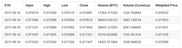
Now, we have a dictionary containing 9 data frames, each of which contains historical daily average price data between Altcoins and Bitcoin.

We can determine whether the data is correct through the last few rows of the Ethereum price table.

altcoin_data['ETH'].tail()

3.3 Unify the currency unit of all price data to USD

Now, we can combine BTC and Altcoins exchange rate data with our Bitcoin price index to calculate the historical price of each Altcoin (in USD) directly.

# Calculate USD Price as a new column in each altcoin data frame
for altcoin in altcoin_data.keys():
    altcoin_data[altcoin]['price_usd'] =  altcoin_data[altcoin]['weightedAverage'] * btc_usd_datasets['avg_btc_price_usd']

Here, we add a new column for each Altcoin data frame to store its corresponding USD price.

To be continued...