The rise of antibiotic resistance rates in Escherichia coli in Europe
I have always been fasciated with using animated graphs to visualise data. It is an attractive way to add another dimension, usually time, to the plot. Animated choropleth map is an effective and only way to present time-series data on a map.
I have no previous experience in making animated plots and would like to start learning/experimenting on them. I do work with R and ggplot2 so making animation based on ggplot2 would be a good start for me. After a bit of research on google, I decided to follow the instructions from this blog as it seems to be most up-to-date and uses many packages I am familiar with.
Here I documented the steps I have taken to make my first animated choropleth map using R. I hope you'll find these codes helpful and reproducible.
The final product of this post is this image:
1. The data
A major focus of my research is on antibiotic resistance of bacteria, especially Escherichia coli. So as a practice for my animiated choroplath map, I dedided to download data from ECDC, showing the average proportion of resistance isolates from European countries every year since 2010 to 2016.
I don't know how to download this data set directly from R so I described here how I downloaded data from ECDC website in a point'n'click way. If you know how to do this in R, please comment to let me know - I would love to learn from you.
- Go to ECDC data website:
- Click on download icon
- Select: (1) All time periods, (2) All regions, (3) All indicators, (4) CSV file
- Click Export to download .csv file (8.7MB)
Alternatively, you can download this csv file here
2. Required packages
The following packages are required for my codes to work. Please note that ggplot2 and gganimate require developer version. See my Extra notes at the bottom for other requirements.
library(tidyverse) # dev ggplot version required:  devtools::install_github("hadley/ggplot2")
library(sf)
library(readxl)
library(gganimate) # devtools::install_github("dgrtwo/gganimate")
3. Load csv file downloaded in step 1 to R
I saved the csv file from step 1 here in my computer:
datafile <- "../ECDC_data/ECDC_surveillance_data_Antimicrobial_resistance.csv"
Load data file with read_csv(), then split column Population into two columns Organisms and Antibiotic using | as a separator.
Notice that I specify the data types for each column in the csv file. This was done by first load the data with read_csv() and let it automatically decide on the data type, review the detected data type and change the read_csv() parameters to proper data type (for example NumValue column will be detected as col_character() and here I changed it to col_double())
d <- read_csv(datafile,
              col_types = cols(
                  HealthTopic = col_character(),
                  Population = col_character(),
                  Indicator = col_character(),
                  Unit = col_character(),
                  Time = col_integer(),
                  RegionCode = col_character(),
                  RegionName = col_character(),
                  NumValue = col_double(),
                  TxtValue = col_character()),
              na = "-") %>%
    separate(col = Population, into = c("Organism","Antibiotics"), sep = "\\|")
The countries included in this data set are:
country.name <- unique(d$RegionName)
country.name
##  [1] "Austria"        "Belgium"        "Bulgaria"       "Cyprus"
##  [5] "Czech Republic" "Germany"        "Denmark"        "Estonia"
##  [9] "Greece"         "Spain"          "Finland"        "France"
## [13] "Croatia"        "Hungary"        "Ireland"        "Iceland"
## [17] "Italy"          "Lithuania"      "Luxembourg"     "Latvia"
## [21] "Malta"          "Netherlands"    "Norway"         "Poland"
## [25] "Portugal"       "Romania"        "Sweden"         "Slovenia"
## [29] "Slovakia"       "United Kingdom"
4. Reduce the data set
In this map, I only want to focus on E. coli so I will filter the data to keep only E. coli. The indicator I would like to display is Resistant (R) isolates proportion so I'll also get rid of other indicators. Several unused columns will also be removed.
# I created this abname object to replace the value in the data with the new value, which are shorter and fit the plot.
abname <- tribble(~current, ~new,
                  "Aminoglycosides", "Aminoglycosides",
                  "Aminopenicillins", "Aminopenicillins",
                  "Carbapenems", "Carbapenems",
                  "Combined resistance (third-generation cephalosporin, fluoroquinolones and aminoglycoside)", "3rdgen-cep/FQ/AMG",
                  "Fluoroquinolones", "Fluoroquinolones",
                  "Third-generation cephalosporins", "3rdgen cep")

# reduce data set
clean_dat <- d %>%
    filter(Organism == "Escherichia coli", Indicator == "Resistant (R) isolates proportion") %>%
    left_join(abname, by = c("Antibiotics"= "current")) %>%
    select(-HealthTopic, -Unit, -TxtValue, -Antibiotics) %>%
    rename(Antibiotics = new)
5. Download the country shapefile from Natural Earth
The shapefiles from Natural Earth are freely available. There are many versions but I find this version contains all the countries in this data set.
shapefile <- "ne_10m_admin_0_countries.shp"

if (!file.exists(shapefile)) {
    # download the natural earth shapefile we need into the working directory
    URL <- "http://www.naturalearthdata.com/http//www.naturalearthdata.com/download/10m/cultural/ne_10m_admin_0_countries.zip"
    temp <- tempfile()
    download.file(URL, temp)
    unzip(temp)
    unlink(temp)
}
6. Load shape file into R with st_read()
Next I read the shape file into R as in sf object and set the projection. I have to admit I do you understand much about the st_transform() function and the syntax for crs = "+proj=longlat +datum=WGS84".
world <- st_read(shapefile) %>%
    st_transform(crs = "+proj=longlat +datum=WGS84") %>%
    select(NAME, NAME_LONG, geometry) # keep only the fields needed
## Reading layer `ne_10m_admin_0_countries' from data source `/Users/uqmphan1/MyWork/Post-doc/Labbooks/Bioinformatics/ABR_mapviz/ECDC_mapviz/ne_10m_admin_0_countries.shp' using driver `ESRI Shapefile'
## Simple feature collection with 255 features and 71 fields
## geometry type:  MULTIPOLYGON
## dimension:      XY
## bbox:           xmin: -180 ymin: -90 xmax: 180 ymax: 83.6341
## epsg (SRID):    4326
## proj4string:    +proj=longlat +datum=WGS84 +no_defs
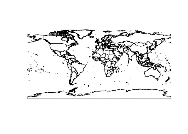
Because sf library works with base plot, we can do a quick check with base plot() function to make sure we have successfully download the shapes.
plot(world$geometry)
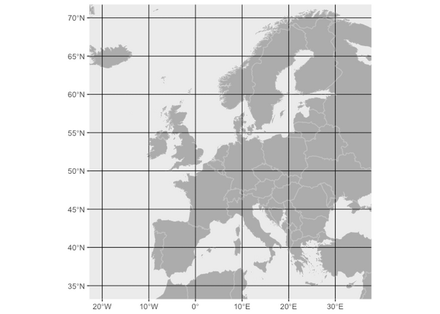
We can also do a quick plot in ggplot2 to check using a new geom: geom_sf (dev ggplot2 version required). Here we set coord_sf(xlim = c(-20,35), ylim = c(35,70)) to view only Europe.
eu_map <- ggplot() +
  geom_sf(data = world, colour = "#ffffff20", fill = "#2d2d2d60", size = .5) +
    coord_sf(xlim = c(-20,35), ylim = c(35,70))
eu_map
7. Combine resistance data with shape data
Before binding resistance data to map data, it is a good idea to check whether the country names in resistance data matched with the country names used in shape data (if you don't use the exact shape file as I do).
match(country.name, world$NAME)
##  [1]  17  20  24  60  NA  62  65  73  91  72  75  78 100 102 108 111 113
## [18] 137 138 139 151 169 170 183 186 191 216 215 214  82
match(country.name, world$NAME_LONG)
##  [1]  17  20  24  60  61  62  65  73  91  72  75  78 100 102 108 111 113
## [18] 137 138 139 151 169 170 183 186 191 216 215 214  82
The following name Czech Republic does not match with world$NAME. We'll have to use the world$NAME_LONG column to match with country names in resistance data.
ecdc_dat <- merge(world, clean_dat, by.x = "NAME_LONG", by.y = "RegionName")
Change Antibiotics column into factors to control the order of facets in the final plot.
ecdc_dat$Antibiotics <- factor(ecdc_dat$Antibiotics, levels = c("Aminopenicillins", "Aminoglycosides", "Fluoroquinolones", "3rdgen cep", "Carbapenems", "3rdgen-cep/FQ/AMG"))
8. Create plot with ggplot
First, I repeat the europe map as in step 6 with geom_sf to set the first layer with background country shapes. Then I added another geom_sf with resistance data (ecdc_dat), connecting fill = NumValue, and to prepare for the animation, I needed to add two more parameters: frame = Time and cumulative = FALSE. These two parameters are not recognised by ggplot2 and thus I expected a warning message from ggplot2.
I also use facet_wrap to separate the data by Antibiotics.
ecdc_res_map <- ggplot() +
    geom_sf(data = world, colour = "#ffffff20", fill = "#2d2d2d60", size = .5) +
    geom_sf(data = ecdc_dat, aes(fill = NumValue, frame = Time, cumulative = FALSE)) +
    scale_fill_gradient(name = "Resistance %", low = "green", high = "red", na.value = "#ffffff20") +
    coord_sf(xlim = c(-20,35), ylim = c(35,70)) +
    facet_wrap(~Antibiotics, ncol = 3) +
    theme_light()
## Warning: Ignoring unknown aesthetics: frame, cumulative
9. Make animated map
I used gganimate to make animated map and saved it to a gif file. See my Extra notes on convert parameter. I set the delay between frame at interval = 0.5. The title_frame = TRUE is set to allow the display of the year corresponding to each frame.
animation::ani.options(interval = 0.5)
gganimate(ecdc_res_map, ani.width =  800, ani.height = 600, filename = "ecdc_res_map.gif", title_frame = TRUE, convert = "gm convert")
## Executing:
## gm convert -loop 0 -delay 50 Rplot1.png Rplot2.png Rplot3.png
##     Rplot4.png Rplot5.png Rplot6.png Rplot7.png Rplot8.png
##     Rplot9.png Rplot10.png Rplot11.png Rplot12.png Rplot13.png
##     Rplot14.png Rplot15.png Rplot16.png Rplot17.png
##     'ecdc_res_map.gif'
## Output at: ecdc_res_map.gif
With this map, we can see the increasing resistance rates in European countries over time. The map is quite basic. If you have any suggestion to make it look better, please comment below.
Extra notes {#notes}
To make animated plots and export to gif format, you'll need to install either ImageMagick or GraphicsMagick to your system.
For ImageMagick, use convert = "convert" in gganimate(). For GraphicsMagick, use convert = "gm convert".
Session Info
sessionInfo()
## R version 3.4.3 (2017-11-30)
## Platform: x86_64-apple-darwin15.6.0 (64-bit)
## Running under: macOS High Sierra 10.13.3
##
## Matrix products: default
## BLAS: /Library/Frameworks/R.framework/Versions/3.4/Resources/lib/libRblas.0.dylib
## LAPACK: /Library/Frameworks/R.framework/Versions/3.4/Resources/lib/libRlapack.dylib
##
## locale:
## [1] en_AU.UTF-8/en_AU.UTF-8/en_AU.UTF-8/C/en_AU.UTF-8/en_AU.UTF-8
##
## attached base packages:
## [1] stats     graphics  grDevices utils     datasets  methods   base
##
## other attached packages:
##  [1] bindrcpp_0.2         gganimate_0.1.0.9000 readxl_1.0.0
##  [4] sf_0.6-0             forcats_0.3.0        stringr_1.3.0
##  [7] dplyr_0.7.4          purrr_0.2.4          readr_1.1.1
## [10] tidyr_0.8.0          tibble_1.4.2         ggplot2_2.2.1.9000
## [13] tidyverse_1.2.1
##
## loaded via a namespace (and not attached):
##  [1] tidyselect_0.2.4  reshape2_1.4.3    haven_1.1.1
##  [4] lattice_0.20-35   colorspace_1.3-2  htmltools_0.3.6
##  [7] base64enc_0.1-3   yaml_2.1.17       rlang_0.2.0.9000
## [10] e1071_1.6-8       pillar_1.2.1      foreign_0.8-69
## [13] glue_1.2.0        withr_2.1.1.9000  DBI_0.7
## [16] modelr_0.1.1      bindr_0.1         plyr_1.8.4
## [19] munsell_0.4.3     gtable_0.2.0      cellranger_1.1.0
## [22] rvest_0.3.2       psych_1.7.8       evaluate_0.10.1
## [25] labeling_0.3      knitr_1.20        class_7.3-14
## [28] parallel_3.4.3    broom_0.4.3       Rcpp_0.12.15
## [31] udunits2_0.13     scales_0.5.0.9000 backports_1.1.2
## [34] classInt_0.1-24   jsonlite_1.5      mnormt_1.5-5
## [37] hms_0.4.1         digest_0.6.15     stringi_1.1.6
## [40] animation_2.5     grid_3.4.3        rprojroot_1.3-2
## [43] cli_1.0.0         tools_3.4.3       magrittr_1.5
## [46] lazyeval_0.2.1    crayon_1.3.4      pkgconfig_2.0.1
## [49] xml2_1.2.0        lubridate_1.7.3   assertthat_0.2.0
## [52] rmarkdown_1.8     httr_1.3.1        rstudioapi_0.7
## [55] R6_2.2.2          units_0.5-1       nlme_3.1-131.1
## [58] compiler_3.4.3