Data Visualization with Python -- GeoSpatial!

0.0 Setup

This guide was written in Python 3.6.

0.1 Python and Pip

If you haven't already, download Python and Pip.

0.2 Libraries

pip3 install geojsonio
pip3 install geopandas
pip3 install shapely
pip3 install descartes 
pip3 install plotly
pip3 install geocoder
pip3 install fiona

0.3 Plotly

We'll be using plotly for some of our visualizations, so sign up and make an account here.

0.4 Data

You can download all the data for this workshops here.

Cool, now we're ready to start!

1.0 Background

1.1 What is Geospatial Data Analysis?

Geospatial analysis involves applying statistical analysis to data which has a geographical or geometrical aspect. In this tutorial we'll review the basics of acquiring geospatial data, handling it, and visualizing it.

1.2 Why is Geospatial Analysis Important?

Think about how much data contains location as an aspect. Anything in which location makes a difference or can be represented by location is likely going to be a geospatial problem. With different computational tools, we can create beautiful and meaningful visualizations that tell us about how location affects a given trend.

1.3 Terminology

Before we get into the specifics, first we'll review some terminology that you should keep in mind.

1.3.1 Interior Set

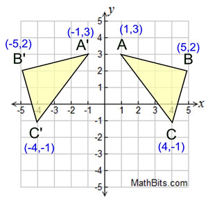
An Interior Set is the set of points contained within a geometrical object. If a geometrical object lies on the x-y axis, it contains points inside that object. For example, in the following image, there are two geometric objects and each one contains its own set of interior points. In ABC, its interior set include points like (3,1).

1.3.2 Boundary Set

A Boundary Set is the set of points which form the outline of a geometrical object. Boundary Sets and Interior Sets have no intersection. From the previous image, any point that falls on the lines forming the triangles is in that object's boundary set. In ABC, some of those points include (1,3), (5,2), and (4, -1).

1.3.3 Exterior Set

An Exterior Set is the set of all other points. For example, the point (2,-3) doesn't fall within any geometric object in this example, making it an exterior point.

1.4 Data Types

Spatial data consists of location observations. Spatial data identifies features and positions on the Earth’s surface and is ultimately how we put our observations on the map.

1.4.1 Point

A Point is a zero-dimensional object representing a single location. Put more simply, they're XY coordinates. Because points are zero-dimensional, they contain exactly one interior point, 0 boundary points, and infinite many exterior points.

1.4.2 Polygon

A Polygon is a two-dimensional surface stored as a sequence of points defining the exterior. The example from the previous section is an example of a polygon!

1.4.3 Curve

A Curve has an interior set consisting of the infinitely many points along its length, a boundary set consisting of its two end points, and an exterior set of all other points.

1.4.4 Surface

A Surface has an interior set consisting of the infinitely many points within, a boundary set consisting of one or more Curves, and an exterior set of all other points.

Surfaces have infinite many interior, exterior, and boundary points.

2.0 Geojsonio and Geopandas

GeoJSON is a specific format for representing a variety of geographic objects. It supports the following geometry types: Point, LineString, Polygon, MultiPoint, MultiLineString, MultiPolygon, and GeometryCollection.

2.1 Geojsonio

Geojsonio is a tool used for visualizing geojson. Here we read in the geojson of a point and plot it on an interactive map.

from geojsonio import display

with open('map.geojson') as f:
    contents = f.read()
    display(contents)

2.2 Geopandas

GeoPandas is a python module used to make working with geospatial data in python easier by extending the datatypes used by pandas to allow spatial operations on geometric types. So now that we know what polygons are, we can set up a map of the United States using data of the coordinates that shape each state.

import geopandas as gpd
import geojsonio

states = gpd.read_file('states.geojson')
geojsonio.display(states.to_json())

3.0 Shapely and Descartes

Shapely converts feature geometry into GeoJSON structure and contains tools for geometry manipulations. This module works with three of the types of geometric objects we discussed before: points, curves, and surfaces. Descartes works off of shapely for visualizing geometric objects!

First, we import the needed modules.

from shapely.geometry import shape, LineString, Point
from descartes import PolygonPatch
import fiona
import matplotlib.pyplot as plt

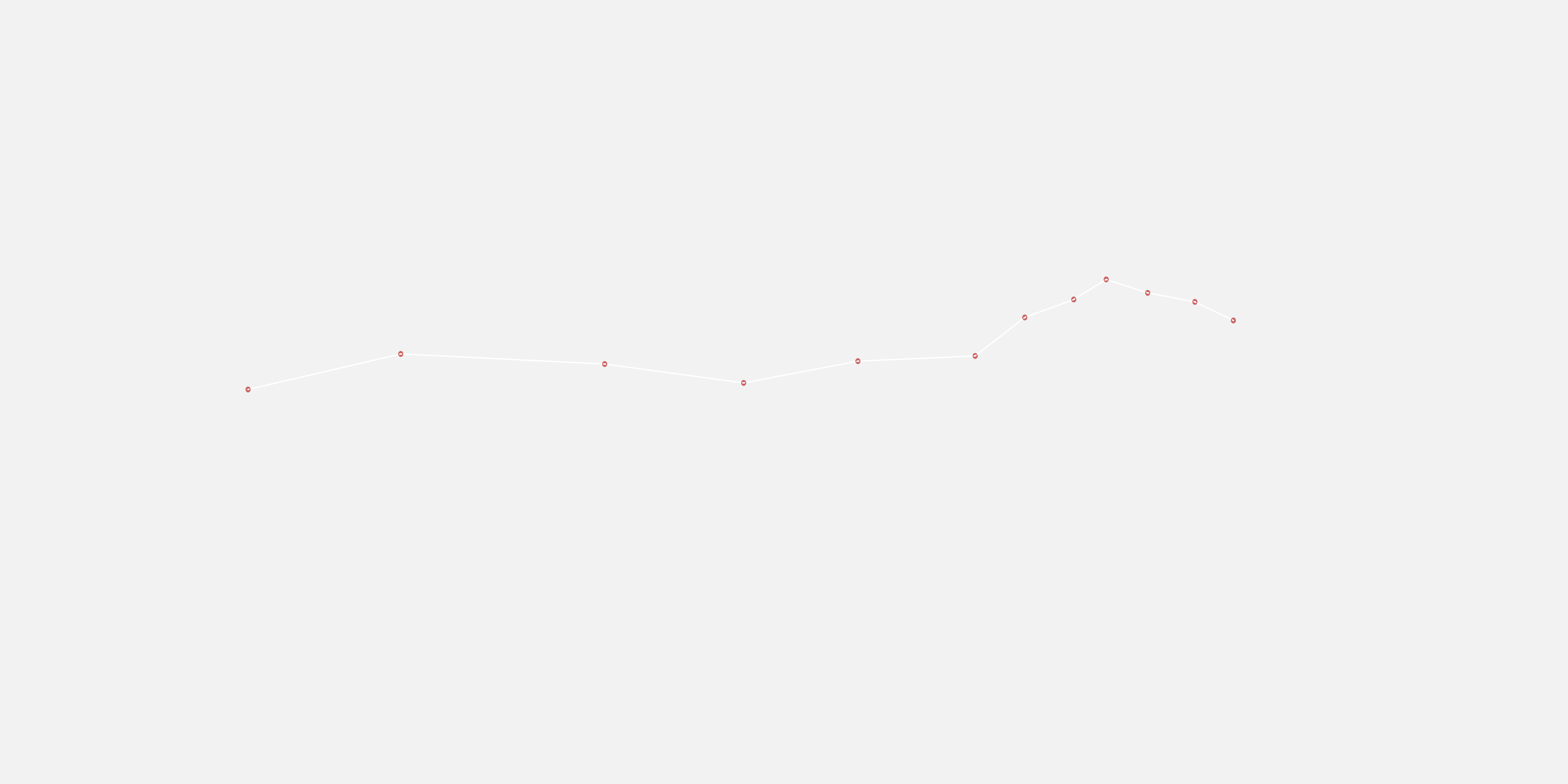
These are some coordinates we'll need to plot the path of a flight from San Francisco to New York.

latlons = [(37.766, -122.43), (39.239, -114.89), (38.820, -104.82), (38.039, -97.96),
    (38.940, -92.32), (39.156, -86.53), (40.749, -84.08), (41.494, -81.66),
    (42.325, -80.06), (41.767, -78.01), (41.395, -75.68), (40.625, -73.780)]

This simply takes the points and reformats the x and y (since it's originally coordinates) and converts it to a LineString type.

path = [(x, y) for y, x in latlons]
ls = LineString(path)

So now we want to display this on a map. Using some data I found online (which you can access via the github), I turn each of these into polygon with fiona.

with fiona.collection("shapefiles/statesp020.shp") as features:
        states = [shape(f['geometry']) for f in features]

fig = pylab.figure(figsize=(24, 12), dpi=180)

Don't worry about this section too much, but it basically finds where the intersections occur to denote a dark outline.

for state in states:
    if state.geom_type == 'Polygon':
        state = [state]

    for poly in state:
        if ls.intersects(poly):
            alpha = 0.4
        else:
            alpha = 0.4

        try:
            poly_patch = PolygonPatch(poly, fc="#6699cc", ec="#6699cc", alpha=alpha, zorder=2)
            fig.gca().add_patch(poly_patch)
        except:
            pass

Here, we format the specifics of our plot.

fig.gca().plot(*ls.xy, color='#FFFFFF')

This is where we set the outlines to a separate color.

for x, y in path:
    p = Point(x, y)
    spot = p.buffer(.1)
    x, y = spot.exterior.xy
    plt.fill(x, y, color='#cc6666', aa=True)
    plt.plot(x, y, color='#cc6666', aa=True, lw=1.0)

And finally, we save this image we have created to a file with a png extension.

fig.gca().axis([-125, -65, 25, 50])
fig.gca().axis('off')
fig.savefig("states.png", facecolor='#F2F2F2', edgecolor='#F2F2F2')

Which should get you something like this:

Resources

If you want to learn more about this topic, check out the resources below, my GitHub, and stay tuned for more!

GeoJSON

OpenStreetMap

CartoDB