Text Mining/Analysis In The R Programming Language On Cancer Survivor Stories

Hi there. In this post, the R programming language is used to conduct text mining/analysis on cancer survivor stories. This particular project is something that I am proud of and I find this topic interesting and motivating. I hope that you as a reader will find the contents and results of this page to be interesting.

Topics in the post include wordclouds, word counts, bigrams (two-word phrases) and sentiment analysis for determining if the stories are positive or negative.

This post does not contain the full code and sections where I remove weird characters such as ’. The full version of this with complete code can be found here at this link: http://dkmathstats.com/using-r-programming-for-text-mining-analysis-on-cancer-survivor-stories/

Image Source

Sections

---

• Introduction
• Wordclouds On Most Common Words
• Word Counts In Cancer Survivor Stories - A tidyttext Approach
• Bigrams In The Cancer Survivor Stories
• Sentiment Analysis
• References / Resources

Introduction

---

In the R programming language, I load in the appropriate packages which allows for data cleaning, data manipulation, text mining, text analysis and plotting (data visualization).

The cancer survivor stories are taken from Cancer Treatment Centers Of America (CTCA) at the website cancercenter.com. These stories are taken from the cancer survivor themselves. In the pages, there are some subheadings and titles which were not copied. Only the stories themselves are copied and pasted to a text file called cancer_survivor_stories.txt.

This text file is read into R with the file() and readLines() functions. Remember to set your working directory to the folder where the text file is.

Note that some of the pages contain more than one cancer survivor story. The types of cancers from the survivor stories do vary. The types of the cancers that are out there include:

• Leukemia
• Breast Cancer
• Prostate Cancer
• Lung Cancer
• Stomach Cancer
• Brain Cancer
• Ovarian Cancer
• Bladder Cancer
• Colorectal Cancer

# Text Mining on Cancer Survivor Stories

# Source: Cancer Treatment Centers Of America (CTCA)
# Website: https://www.cancercenter.com/community/survivors/
# About 125 stories
# No titles but the stories from the survivors themselves. Some pages have two stories instead of one.
# Different types of cancers represented from survivors.

# 1) Wordclouds
# 2) Word Counts (Check For themes)
# 3) Bigrams (Two Word Phrases)
# 4) Sentiment Analysis - Are the stories positive or negative?

#----------------------------------

# Load libraries into R:
# Install packages with install.packages("pkg_name")

library(dplyr)
library(tidyr)
library(ggplot2)
library(tidytext)
library(wordcloud)
library(stringr)
library(tm)

# Reference: https://stackoverflow.com/questions/12626637/reading-a-text-file-in-r-line-by-line

fileName <- "cancer_survivor_stories.txt"
conn <- file(fileName, open = "r")
linn <- readLines(conn)

# Preview text:
for (i in 1:length(linn)){
print(linn[i])
}
close(conn)

Wordclouds On Most Common Words

---

In this section, I use R to generate wordclouds on the most common words. The survivor_stories object is put into the VectorSource() function and that is put is into the Corpus() function.

Once you have the Corpus object, the tm_map() functions can be used to clean up the text. In the code below, I convert the text to lowercase, remove numbers and strip whitespace.

# 1) Wordclouds
# Reference: http://www.sthda.com/english/wiki/text-mining-and-word-cloud-fundamentals-in-r-5-simple-steps-you-should-know

cancerStories_text <- Corpus(VectorSource(linn))


survivor_stories_clean <- tm_map(cancerStories_text, content_transformer(tolower))
survivor_stories_clean <- tm_map(survivor_stories_clean, removeNumbers)
survivor_stories_clean <- tm_map(survivor_stories_clean, stripWhitespace)
In tm_map(), you can remove English stopwords such as and, the, of, much, me, myself, you, etc. Add in the options removeWords and stopwords('english').

From investigation of the texts, there is this weird ’ thing which is there instead of the apostrophe in words like don't, they're and won't. This strange thing is removed in the code later below.

# Remove English stopwords such as: the, and or, over, under, and so on:

> head(stopwords("english"), n = 15) # Sample of English stopwords
 [1] "i" "me" "my" "myself" "we" "our" 
 [7] "ours" "ourselves" "you" "your" "yours" "yourself" 
[13] "yourselves" "he" "him" 

survivor_stories_clean <- tm_map(survivor_stories_clean, removeWords, stopwords('english'))
Now, the stories are converted in a term document matrix and then in a data frame.

# Convert to Term Document Matrix:

dtm <- TermDocumentMatrix(survivor_stories_clean)
m <- as.matrix(dtm)
v <- sort(rowSums(m),decreasing=TRUE)
d <- data.frame(word = names(v),freq=v)

#Preview data:
head(d, n = 20)
 word freq
cancer cancer 1393
ctca ctca 1242
treatment treatment 1067
care care 693
time time 603
also also 441
chemotherapy chemotherapy 388
one one 375
life life 345
told told 345
surgery surgery 344
doctor doctor 336
first first 322
hospital hospital 322
day day 312
felt felt 312
team team 285
just just 279
years years 279
like like 279

---

Now that the data is cleaned up, wordclouds can be generated with the wordcloud() functions.

# Wordcloud with colours:

set.seed(1234)
wordcloud(words = d$word, freq = d$freq, min.freq = 100,
max.words = 200, random.order=FALSE, rot.per=0.35, 
colors = rainbow(30))

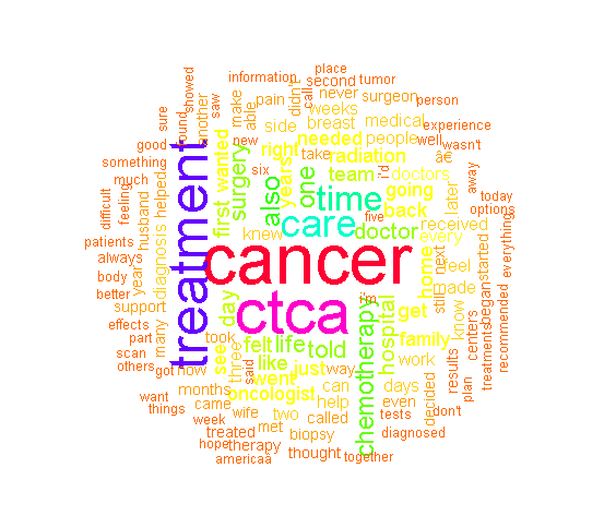
This particular wordcloud is quite big and contains a good variety of words. The most common words include cancer, treatment, ctca, care as those words are the largest in the wordcloud. (There is this †thing in the wordcloud which was not removed.)

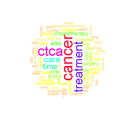
To achieve a smaller wordcloud, you can raise the minimum frequency and lower the maximum words inside the wordcloud() function.

# Wordcloud with colours with lower max words and raise minimum frequency:

wordcloud(words = d$word, freq = d$freq, min.freq = 150,
          max.words=120, random.order=FALSE, rot.per=0.35, 
          colors = rainbow(30))

---

From all the tm_map() preprocessing and obtaining the dataframe from the term document matrix, we can display the most common words with the use of the ggplot2 package. The mutate() function is used to sort the words from the most common word to the least common word from the stories. Aesthetic add-on functions in ggplot2 include labs(), theme() and geom_text().

# ggplot2 bar plot:

d[1:30, ] %>% 
mutate(word = reorder(word, freq)) %>% 
ggplot(aes(word, freq)) + 
geom_col(fill = "darkgreen") +
coord_flip() +
labs(x = "Word \n", y = "\n Count ", title = "Word Counts In \n Cancer Survivor Stories \n") +
geom_text(aes(label = freq), hjust = 1.2, colour = "white", fontface = "bold", size = 3.7) +
theme(plot.title = element_text(hjust = 0.5), 
axis.title.x = element_blank(),
axis.ticks.x = element_blank())

---

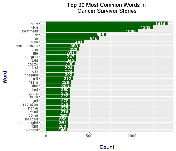
The top word from the stories is cancer. The second common word is ctca which refers to the Cancer Treatment Centers Of America (CTCA). Other notable common words which are related to the topic of cancer include:

• treatment
• care
• chemotherapy
• surgery
• doctor
• hospital
• radiation
• oncologist

Word Counts In Cancer Survivor Stories - A tidytext approach

---

The previous section had a sideways bar graph of the most common words with the use of tm_map(). This section looks at word counts from the tidytext approach. The main reference book is Text Mining With R - A Tidy Approach by Julia Silge and David Robinson.

### 2) Word Counts In Survivor Stories - A tidytext approach

survivor_stories <- readLines("cancer_survivor_stories.txt")

# Preview the stories:

survivor_stories_df <- data_frame(Text = survivor_stories) # tibble aka neater data frame

> head(survivor_stories_df , n = 20)
# A tibble: 20 x 1
 Text
 <chr>
 1 I was born and raised in a small town on Long Island in New York. I live there today with m
 2 
 3 One day in September 2015, I felt a lump in my left breast. I am not an alarmist, but I am 
 4 
 5 I have known my doctor for years, since she delivered my children. During my exam, she agre
 6 
 7 Since I didn’t know any surgeons, I was referred to one. I saw the surgeon the very next 
 8 
 9 I felt my world spinning. I barely remember the rest of the phone call. My mind was going a
10 
11 I went in the very next week to meet with the surgeon. He did an MRI on both of my breasts.
12 
13 My husband and I met with an oncologist that the surgeon referred us to within his same pra
14 
15 I started doing some research about other options. Then I called my friend who was a cancer
16 
17 The next day, a representative called and we scheduled my initial evaluation. The represent
18 
19 I came to CTCA with my husband. We stayed at a hotel close by, and we used a shuttle service
20

---

Next, the unnest_tokens() function from the tidytext R package is used. This will convert the words in the text file in a way such that each row has one word.

# Unnest tokens: each word in the stories in a row:

survivor_words <- survivor_stories_df %>% 
unnest_tokens(output = word, input = Text)

# Preview with head() function:

> head(survivor_words, n = 10)
# A tibble: 10 x 1
 word
 <chr>
 1 i
 2 was
 3 born
 4 and
 5 raised
 6 in
 7 a
 8 small
 9 town
10 on

---

In any piece of text, there are words in the English language which makes sentences flow but carry no/little meaning on their own. These words are called stop words. Examples include the, and, me, you, that, this.

R's dplyr function provides the count() function for obtaining word counts for each word.

---

# Remove English stop words from the cancer survivors stories:
# Stop words include the, and, me , you, myself, of, etc.

survivor_words <- survivor_words %>%
anti_join(stop_words)

# Word Counts:

survivor_wordcounts <- survivor_words %>% count(word, sort = TRUE)

> head(survivor_wordcounts, n = 15)
# A tibble: 15 x 2
 word n
 <chr> <int>
 1 cancer 1408
 2 ctca 1242
 3 treatment 1068
 4 care 695
 5 time 615
 6 chemotherapy 388
 7 life 350
 8 surgery 346
 9 told 345
10 doctor 337
11 day 323
12 hospital 322
13 team 286
14 home 275
15 radiation 275
> 
> print(survivor_wordcounts[16:30, ])
# A tibble: 15 x 2
 word n
 <chr> <int>
 1 oncologist 250
 2 family 240
 3 doctors 237
 4 received 218
 5 diagnosis 215
 6 breast 205
 7 days 200
 8 feel 197
 9 people 195
10 weeks 194
11 medical 193
12 called 181
13 helped 174
14 months 174
15 pain 160

---

Results of the word counts can be plotted with the use of ggplot2 graphics and functions.

survivor_wordcounts[1:30, ] %>% 
 mutate(word = reorder(word, n)) %>% 
 ggplot(aes(word, n)) + 
 geom_col(fill = "red") +
 coord_flip() +
 labs(x = "Word \n", y = "\n Count ", title = "Top 30 Most Common Words In \n Cancer Survivor Stories \n") +
 geom_text(aes(label = n), hjust = 1, colour = "white", fontface = "bold", size = 3.5) +
 theme(plot.title = element_text(hjust = 0.5), 
 axis.ticks.x = element_blank(),
 axis.title.x = element_text(face="bold", colour="darkblue", size = 12),
 axis.title.y = element_text(face="bold", colour="darkblue", size = 12))

---

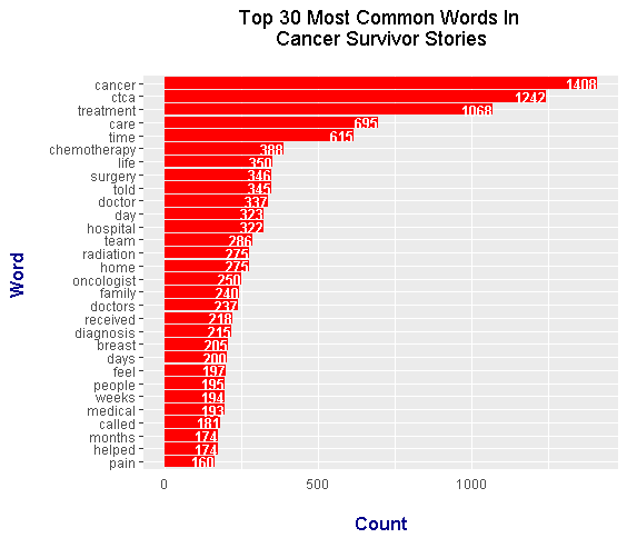
Although the top two common words are cancer and ctca, this most common words bar graph is slightly different from the one in the previous section. Notable common words that are related to cancer include:

• treatment
• care
• chemotherapy
• surgery
• doctor
• hospital
• team
• oncologist
• doctors
• diagnosis
• breast
• medical
• pain

This tidytext approach bar graph on common words includes the words breast, diagnosis, medical and pain.

Bigrams In The Cancer Survivor Stories

---

The previous section looked at the most common single words. This section looks at the most common bigrams (two-word phrases) in the cancer survivor stories.

### 3) Bigrams (Two-Word Phrases) in Remember The Name:

survivor_bigrams <- survivor_stories_df %>% 
unnest_tokens(bigram, input = Text, token = "ngrams", n = 2)

# Look at the bigrams:

> survivor_bigrams
# A tibble: 149,661 x 1
 bigram
 <chr>
 1 i was
 2 was born
 3 born and
 4 and raised
 5 raised in
 6 in a
 7 a small
 8 small town
 9 town on
10 on long
# ... with 149,651 more rows

Like in the single words, the stop words need to be removed from the bigrams. Removing the stopwords in bigrams takes a little bit more work. R's tidyr package and its separate function will be used here. The separate() function will split the bigram into two separate words, the filter() functions will keep the words that are not stop words from each of the two separate words and the count() function will give counts.

# Remove stop words from bigrams with tidyr's separate function
# along with the filter() function

survivor_bigrams_sep <- survivor_bigrams %>%
separate(bigram, c("word1", "word2"), sep = " ")

survivor_bigrams_filt <- survivor_bigrams_sep %>%
filter(!word1 %in% stop_words$word) %>%
filter(!word2 %in% stop_words$word)

# Filtered bigram counts:
survivor_bigrams_counts <- survivor_bigrams_filt %>% 
count(word1, word2, sort = TRUE)

> head(survivor_bigrams_counts, n = 15)
# A tibble: 15 x 3
 word1 word2 n
 <chr> <chr> <int>
 1 cancer treatment 215
 2 care team 160
 3 treatment centers 136
 4 americaã‚ ctca 111
 5 i㢠ve 93
 6 breast cancer 90
 7 medical oncologist 69
 8 lymph nodes 61
 9 treatment plan 58
10 cancer diagnosis 49
11 ct scan 45
12 treatment options 44
13 oncology information 40
14 radiation therapy 40
15 radiation treatment 40

---

Now that the counts are obtained, the separated words can be gathered together with the use of the unite() function from R's tidyr package.

# Unite the words with the unite() function:

survivor_bigrams_counts <- survivor_bigrams_counts %>%
unite(bigram, word1, word2, sep = " ")

> survivor_bigrams_counts
# A tibble: 8,646 x 2
 bigram n
 * <chr> <int>
 1 cancer treatment 215
 2 care team 160
 3 treatment centers 136
 4 americaã‚ ctca 111
 5 i㢠ve 93
 6 breast cancer 90
 7 medical oncologist 69
 8 lymph nodes 61
 9 treatment plan 58
10 cancer diagnosis 49
# ... with 8,636 more rows

---

In the bigrams, there is americaã‚ ctca with the weird character ã and i㢠ve. (The code for removing the ã is not shown here.)

With the use of R's ggplot2 package, a bar graph of the bigrams can be produced.

# We can now make a plot of the word counts.
# ggplot2 Plot Of Top 20 Bigrams From Cancer Stories:

survivor_bigrams_counts[1:20, ] %>% 
ggplot(aes(reorder(bigram, n), n)) + 
geom_col(fill = "darkgray") +
coord_flip() +
labs(x = "Bigram \n", y = "\n Count ", title = "Top 20 Bigrams In \n Cancer Survivor Stories \n") +
geom_text(aes(label = n), hjust = 1.2, colour = "black", fontface = "bold") +
theme(plot.title = element_text(hjust = 0.5), 
axis.title.x = element_blank(),
axis.ticks.x = element_blank(),
axis.text.x = element_blank(),
axis.title.y = element_text(face="bold", colour="darkblue", size = 12))

---

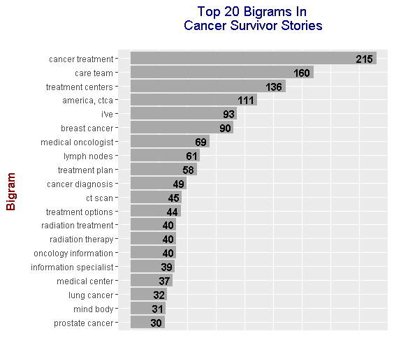
From the results, top bigrams include:

• cancer treatment
• care team
• treatment centers
• breast cancer
• medical oncologist
• lymph nodes
• treatment plan
• cancer diagnosis
• ct scan
• radiation treatment
• radiation therapy

Sentiment Analysis

---

(I will show the code for the nrc Lexicon only and the outputs for all three nrc, bing and AFINN lexicons.)

Sentiment analysis looks at a piece of text and determines whether the text is positive or negative. The lexicons determine the positivity or negativity of a piece of text. Three main lexicons are used in this analysis. The three lexicons are:

• nrc
• bing
• AFINN

These lexicons are highly subjective and are not perfect. For more information of these lexicons, please refer to section 2.1 of Text Mining With R with Julia Silge and David Robinson.

Website Link: https://www.tidytextmining.com/sentiment.html

nrc Lexicon

The nrc lexicon categorizes words with the sentiment of either:

• trust
• fear
• negative
• sadness
• anger
• positive
• negative

From the nrc lexicon, the sentiments of interest are positive and negative. From the survivor_wordcounts object, an inner_join is used to match the words with the nrc sentiment words. A filter() function is used to extract words with a positive or negative sentiment from the nrc lexicon.

Note that the word_labels_nrc part is for the labels in the facet_wrap() add on function. This yields the labels Negative Words and Positive Words in the plot below.

# 4) Sentiment Analysis 
# Are the stories positive, negative, neutral?

# Using nrc, bing and AFINN lexicons

word_labels_nrc <- c(
`negative` = "Negative Words",
`positive` = "Positive Words"
)

### nrc lexicons:
# get_sentiments("nrc")

survivor_words_nrc <- survivor_wordcounts %>%
inner_join(get_sentiments("nrc"), by = "word") %>%
filter(sentiment %in% c("positive", "negative"))

> head(survivor_words_nrc)
# A tibble: 6 x 3
 word n sentiment
 <chr> <int> <chr>
1 cancer 1408 negative
2 doctor 337 positive
3 radiation 275 negative
4 received 218 positive
5 diagnosis 215 negative
6 medical 193 positive

---

A horizontal bar graph is produced for words with a count over 70 from the cancer survivor stories.

# Sentiment Plot with nrc Lexicon (Word Count over 70)

survivor_words_nrc %>%
filter(n > 70) %>%
ggplot(aes(x = reorder(word, n), y = n, fill = sentiment)) + 
geom_bar(stat = "identity", position = "identity") +
geom_text(aes(label = n), colour = "black", hjust = 1, fontface = "bold", size = 3) +
facet_wrap(~sentiment, nrow = 2, scales = "free_y", labeller = as_labeller(word_labels_nrc)) +
labs(x = "\n Word \n", y = "\n Word Count ", title = "Negative & Positive Words \n In The Cancer Survivor Stories \n With The nrc Lexicon \n") +
theme(plot.title = element_text(hjust = 0.5), 
axis.title.x = element_text(face="bold", colour="darkblue", size = 12),
axis.title.y = element_text(face="bold", colour="darkblue", size = 12),
strip.background = element_rect(fill = "#8DECC7"),
strip.text.x = element_text(size = 11, face = "bold"),
strip.text.y = element_text(size = 11, face = "bold")) +
scale_fill_manual(values=c("#FF0000", "#01DF3A"), guide=FALSE) + 
coord_flip()

---

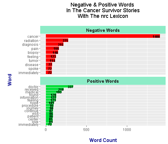
The top negative words include:

• cancer
• radiation
• diagnosis
• pain
• biopsy
• feeling
• tumor
• disease.

It is somewhat weird that the nrc lexicon puts the words feeling, spoke and immediately as negative (even if the lexicons are subjective).

Positive words include doctor, received, medical, found, information, feeling, hope and journey. The words found, received and feeling are more neutral words than positive words. Lexicons do not consider context and are subjective.

bing Lexicon

With the bing lexicon, words are categorized as either positive or negative.

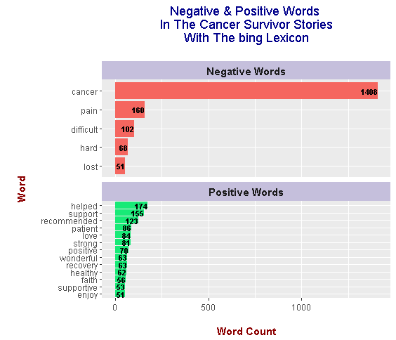
There may be less negative words but the top negative word is still cancer with a count of 1408. Positive words include helped, support, recommended, patient, love, strong and positive. The word patient is probably mislabeled as a positive adjective versus a noun as in a hospital patient.

AFINN Lexicon

In the AFINN lexicon, words are given a score from -5 to +5 (inclusive). Negative scores indicate negative words while positive scores indicate positive words.

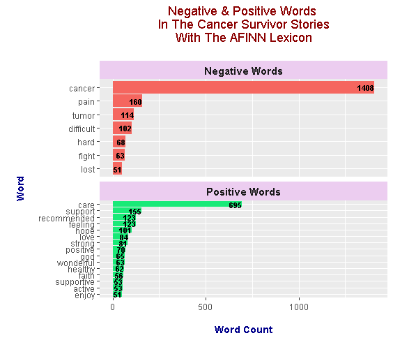
Featured negative words from the AFINN lexicon are cancer, pain, tumor, difficult, hard, fight and lost. Top positive words include care, support, recommended, feeling, hope, strong, positive, healthy, god and faith. I like the AFINN lexicon results as the word care is included. Care plays a big part for those going through cancer treatment.

I am somewhat disappointed in not seeing the word team as the fight against cancer requires more than one person and a very caring and specialized team of health professionals.

References And Resources

---

• https://www.cancercenter.com/community/survivors/
• R Graphics Cookbook By Winston Chang
• https://stackoverflow.com/questions/3472980/ggplot-how-to-change-facet-labels
• Text Mining With R with Julia Silge and David Robinson
• https://stackoverflow.com/questions/13043928/selecting-rows-where-a-column-has-a-string-like-hsa-partial-string-match
• https://stackoverflow.com/questions/24576075/gsub-apostrophe-in-data-frame-r
• http://stat545.com/block022_regular-expression.html
• https://rstudio-pubs-static.s3.amazonaws.com/265713_cbef910aee7642dc8b62996e38d2825d.html

Image Source