Cryptocurrencies - What is the fair value of a currency?
Introduction
In this article, I present a brand new rational model which I have called Currencies Fair Value (CFV). This model can be used to assess the compounded fair value of a currency in terms of another currency. For the first time, thanks to the blockchain technology and to this model, it is feasible to calculate the fair value of a currency. I will show that without making use of any market data at all, one can estimate the price of a blockchain currency in terms of another and the error be very small. The former will be the empirical proof that the model is right. The other proof is the rational proof, which could take us down to praxeology (see Human Action, by Ludwig von Mises).

What is a fair value?
The concept of fair value might sound familiar to an investor. There are two kinds of assets: those whose fair value is intrinsic and those whose fair value can be expressed as a function of intrinsic fair values.
The intrinsic fair value is the function that turns the ordinal preferences of the human minds into a price. Therefore, the price at which an individual buys something ordinary (for instance, a banana) is always smaller or equal to the fair value that the individual assigns to the thing he is buying. When many human beings trade an ordinary good or service, we can refer to the current fair value of that good or service as the price of it. If we were to invest in that ordinary good or service (bananas), we would need to predict the future changes in the scale of preferences of the human minds of the society with regard to that ordinary good or service. We can call this fair value a predicted fair value, a future fair value or a speculated fair value.
We can call compounded fair value to any fair value that can be expressed as a function of intrinsic fair values. Their existence is justified under the rules of rational thinking. If an individual was rational and they were to assess the fair value of a compounded asset, they would first assess the intrinsic fair values of the underlying ordinary assets and then use the rational function to obtain the compounded fair value. Examples of compounded assets with compounded fair values are stocks, bonds, derivatives or currencies. All these things derive their fair values from intrinsic fair values like cash flows, interest rates, ordinary goods and services, or even other compounded fair values (like in the case of financial derivatives).
Predicted fair values are key to investors, for if the investor can predict a correct fair value, the price in the future will converge to their predicted fair value. Some compounded fair values must always be predicted fair values, because the rational thinking implies the necessity to use future intrinsic fair values in its rational function. Discounted Free Cash Flows model or Price to Earnings model are examples of rational functions that use future intrinsic fair values to assess the compounded fair value of a stock.
Rational models can be easier or more complicated, but all of them must have a known intrinsic error, for mapping the praxeological ordinal space to a cardinal space is an heuristic action. Rational models can also suffer from an incorrect or a simplified logic, should it be the case, these models will add a simplification error. Sometimes, simple models have a greater overall error than complex models. In other cases it is the opposite. Moreover, if a model uses future intrinsic fair values, it will be subjected to speculation error.
Some results from CFV
The following charts show the fair value of DASH (Dash) and of LTC (Litecoin) in BTC (Bitcoin), calculated with the CFV model, and their actual historical price:


If the former charts are not impressive, it might be because I have not insisted enough in the fact that fair value does not use any data from any market at all (no prices, no market cap, no order books, etc.) If we combine it with the fact that the fair value depicted in those charts appears to converge to the actual price of the currency, they may look more impressive. In other words, I have pluged some data, not related with the markets, into a rational model for the compounded fair value and, magically, I have arrived to a number very close to the actual price.
How can that be possible? Is not the price something speculative that no one can discover but the market itself? How is it possible to discover the price without looking at the market? Why do the lines appear to converge in the recent months, but not a couple of years ago? I will explain the model and try to answer the questions in the subsequent sections.
The Total Discounted Supply Theory of Money
If no one has heard about the Total Discounted Supply Theory of Money (TDSTM) is because it does not exist (yet). Nonetheless the Quantity Theory of Money (QTM) does exist. The Total Discounted Supply Theory of Money is my modification to the Quantity Theory of Money.
Note: It would more accurate to call them models, rather than theories. From my point of view, an economic theory must work directly with apodictic truths. Whenever we enter the cardinal space, we are developing models, which can be closer or farther from praxeology. This is, they may imitate human action in a better or worse manner. Nonetheless, in order to hold the symmetry with QTM, I will keep the term “theory” within the name of my new model.
What the QTM tries to model is the human action of trading money for goods and services. In its average version, QTM proposes the following:

Where M stands for the money in circulation, V (“velocity of money”) stands for the average number of times a unit of money is traded per unit of time. P stands for the average price of the good or service in each transaction. And T stands for the number of transactions per unit of time (including only the transactions where a good or service was traded). Sometimes this model is used to try find out what the value of the velocity of money is. Other times it is used to try to convince others that if the monetary authority increases M, P – the average price of the goods and services – shall increase. Of course, providing that V and T do not change.
Therefore, the usefulness of the QTM only shows when we establish hypotheses of causality and independence. From now on, I will work with the following hypotheses:
- The velocity of money is independent from the other variables and tied to the human action.
- The average price of goods and services is a consequence of the other variables.
At this point one might be wondering why I decided to modify the QTM. The answer is that current QTM does not account for future increases in the money supply. As simple as it sounds. If there is certainty that in a year the money supply will be doubled by any means of injection procedure, human beings will advance their spending and therefore will stimulate price increases. This simple human reasoning is one of the underlying causes of the hyperinflation phenomenon.
To account for units of currency created in the future, one must discount their nominal value using the time value of money model – another economic model that tries to imitate the consequences of what Ludwig von Mises denominated originary interest –
The modification of QTM introduced by TDSTM is to consider M as the sum of the current supply plus the discounted future supply. It can be expressed as:
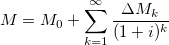
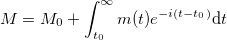
Where M0 stands for the current supply in circulation, i stands for the interest rate, t stands for the time, t0 stands for the current time, ΔMk stands for the future increase of the supply at instant k, and m(t) stands for the velocity of the supply increase. From now on, I will call M the total discounted supply.
One important property of money that TDSTM is able to capture is the fact that present units of money are fungible while future unites are not. No future unit issued at a different instant in the future time is fungible yet. Once a unit of money is issued, it becomes part of the first term of the equation and thus, becomes fungible.
The Currencies Fair Value Model
The cardinal value of something can only be expressed in terms of another thing. There is no such thing as an absolute price. Every price comprises a pair of assets: the priced asset and the reference asset. For instance, one can only say that one car is worth N units of a currency (i.e. USD), but it is impossible to say that the car is worth an absolute number. Everything has a relative value in economy because everything is derived from the ordinal scale of preferences of every individual.
In the former section, I introduced the variable P, and I explained that it represented the average price of the good or service in each transaction. P is just the amount of currency used for buying one unit of the average good or service, and thus, a relative value.
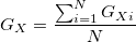
Let GX be the average good or service in each transaction of the currency X, and let GXi be a single good or service traded for the currency X. GXi is a member of the set of assets that are traded for the currency X, that we can call gX. One can express GX in terms of GXi as:
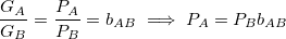
If we have two currencies A and B, it is immediate to establish the following identities, which express the value of the average goods and services with respect to each of the currencies:


If the set of assets traded for the currency A does not match exactly the set of assets traded for the currency B, we will say that their basket is offset proportionally by an amount bAB:

In order to be able to find the value of bAB, one would need to investigate the baskets gA and gB or get the average value of transactions in each of the currencies from the blockchain itself and then convert it to a reference currency that will allow us to obtain bAB directly. That would give us the current value of bAB. Nonetheless, if a currency A aims to substitute a currency B, or both aim to target the same users, their expected bAB should be very close to 1.
In general we can write:
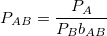
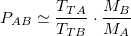
Which means that PA units of currency A can be traded for PB times bAB units of currency B. If we call PAB the price of the currency A in terms of the price of the currency B, we can deduce that:
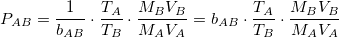
Therefore, using the Total Discounted Supply Theory of Money, the following expression holds true:
It is very important to notice that, given the hypotheses established for QTM and TDSTM, PAB is the compounded fair value of the currency A in terms of the currency B, because PAB becomes a consequence of terms of the right hand side of the equation.
One can either measure or predict the value of every variable in the right hand side of the equation. There are cases where the uncertainty of a variable can be very small, like for example the case of a known supply currency. For other variables, there might be a big speculation (prediction) error. It all depends on the nature of the currency and on the data available.
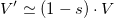
In the case of comparing two non-staking currencies used by or aimed to the same society, and because we are working under the hypothesis that the velocity of money is ruled by the human action, one will not work under a significant error while assuming that:

The velocity of money also accounts for the lost units. That is, units that have been issued but they have become lost forever, because they cannot be recovered by any living individual. To add a little bit of complexity to the problem, we could always try to correct each velocity by imposing a model on how the units of the currency get lost forever. I will leave this to a further analysis and suppose that the proportion of lost units is almost equal in both currencies.
In addition, it is typical, in the case of cryptocurrencies, that we have access to the total number of transactions, but we do not know the percentage of the total transactions that were trades. If we call TT the total number of transactions per unit of time, we can state without loss of generality that:

If we suppose that proportion of transactions that were trades in the currency A (aA) is very similar to the proportion of transactions that were trades in the currency B (aB),
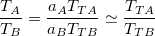
Which leads to a simpler equation for the fair value:
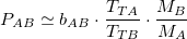
As I indicated before, bAB may be considered to be close to 1 in many circumstances. Should one be considering one of those circumstances, the former equation turns into:
There are important consequences of the Currencies Fair Value model. The value of a currency is directly proportional to the number of trades that are taking place per unit of time. Nonetheless, it is inversely proportional to the total discounted supply and inversely proportional to the velocity of it. Thus, a currency which increases its velocity will lose value with respect to any other currencies whose velocity do not increase that much. In addition, printing money does not sound like a good idea to increase the price of a currency in terms of other currencies.
Using CFV for deriving the fair value of limited supply currencies with exponentially decaying supply increases
If we did not have a clue whatsoever about what the future variations of the supply of a currency would be, and if we just rejected predicting the future by extrapolating past data and there were no other sources where to get the information from, we could still use the future discounted supply presented in the TDSTM. We would just say that:

Of course, if we wanted to track the error that we made while in the whole process of calculating the fair value, we could do it here, as well as in the rest of the cases. For there always be variables which we predict with an error. In order not to make this article very complex and because I found error analysis to be devoid of utility for the main purpose of this article, I have decided to omit it. However, if someone feels in the need to do the error analysis, beware that he will have to deal with non-linear equations and with the integration of errors.
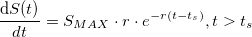
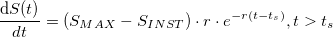
That being said, in the case that we are able to predict the future variations of the supply, even though the predictions could be bounded with an error, we would have knowledge on ΔMk and on m(t). A good example of this is the one of the limited supply cryptocurrencies with an exponentially decreasing supply increases. They usually follow a discrete emission pattern with random time steps whose value follow a Poisson distribution. Because the resolution usually lays within the range of minutes, we can simplify it – and the error be negligible – by approximating it to a continuous distribution model with the following rule for the supply S(t):

Where ts stands for the time at the start of the currency life, r stands for the emission decreasing ratio, and SMAX stands for the theoretical maximum supply that will ever exist.
Taking the first derivative of the supply we get the velocity of the supply (m(t)):
As it is easily seen, it tends to 0 at infinity. Now plugging it into the total discounted supply equation:
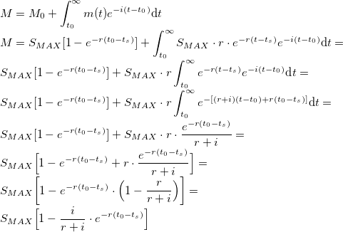
There are two extreme special cases with regarding to the time preference of humans (interest rate): no time preference – people give the same value to future goods and to present goods –, and infinite time preference – people do not give any value to future goods and they just want present goods –. In the first case:

Which, as it can be seen, implies that future money becomes fungible because individuals value future issued units of the currency as much as they value current units of the currency. In the infinite case:

which is just the supply formula along time. Which means that M is just the available supply in circulation, because individuals do not give any value to future units of the currency.
A useful approximation that can be made in the case that one needs to get fast results. If r is much greater than i, if r is big with regard to the time the currency has been around, or if the currency has been around for a considerable time compared with r,

Using CFV for deriving the fair value of staking cryptocurrencies
I call staking cryptocurrencies to a special case of cryptocurrencies, where keeping cash balances instead of spending them is explicitly incentivized. Typically, the reason they are set up that way is to give security to the blockchain (proof-of-stake) and/or to be able to provide additional monetary services.
Stacking has a direct effect on the velocity of money, because it becomes almost certain that a known amount of the currency units have a low probability of being traded and, thus, almost a zero velocity. If we know how many of these units are destined to staking or will be destined to staking, we can correct the velocity of money (V) to that extent. Let s be the proportion of currency units known to be used for staking and ps the probability that a staking unit is traded. We can infer that:
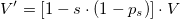
If ps were negligible, which is not an unreasonable assumption, then
Using CFV for deriving the fair value of specific purpose currencies (aka. Tokens)
There are special cases of cryptocurrencies which that required with exclusivity for a special service (typically a service supported by a blockchain). These cryptocurrencies are named tokens. Usually one can obtain, from the blockchain itself, how many of the transactions of the token were trades for the specific service and what was the average value of them. If we were to calculate the fair value of a token (A) in terms of a general-purpose currency (B), finding bAB is all that is needed.
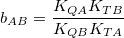
If we work under the hypothesis that all transactions of A but those associated to the specific service share the same basket with B (a generalist currency), and if we can get the number and the amount of the specific service transactions from the blockchain, we can easily calculate the proportion of the specific transactions with respect to all transactions (KT) and the proportion of the specific amounts with respect to all amounts (KQ). bAB can be obtained as follows:

If we were to obtain the fair value of a token (A) in terms of another token B, instead of a generalist currency, then:
Using CFV for deriving the fair value of Dash
In order to assess the fair value of Dash along time we must need to face the following problems:
- Determining the proportion of DASH known to be used for staking (Masternodes collateral).
- Taking into account the instamine event.
- Taking into account never created DASH from the treasury.
As for the proportion of DASH being used for staking, the solution is easy. Because the collateral of each Masternode is 1000 DASH, one only needs to do the following calculation to get the value of s along time:
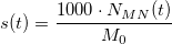
Being NMN(t) the number of Masternodes along time.
The instamine issue has an impact on the total discounted supply (M) along time. The formula for limited supply currencies with exponentially decaying supply increases must be slightly modified in order to account for that event. If we assume that the instamine occurred in a negligible period of time and that the actions taken after it did not modify the emission decreasing ratio (r) in the code of the Dash Core, the supply and the velocity of the supply along time can be written as:

Because the number of the never created DASH from the treasury (SU(t)) is not known in advance, we can only take it into account in the fungible part of the equation. The result for M is the following:

As for the DASH basket, we can assume that it is a general-purpose currency.
Applications
Should the results of CFV be close to reality and, for the experiments I have carried, they are, the amount of applications could be inconceivable. To give some examples:
- It is useful to learn how the price discovery of a currency works.
- It is useful to know when the long-term speculation does not make sense if one cannot predict the relative number of transactions between two currencies.
- It is useful for speculating with a non-monetized currency pair (for instance DASH/USD).
- It can be thought as similar to the rational models we use to obtain the fair value of stocks: Price to Earnings, Discounted Free Cash flows, etc. So it can be at least as useful as these models are.
- It is useful to design the best strategy for a currency to succeed. For instance, one should aim to have billions of transactions instead of transactions of billions. Or one should promote holding, which decreases the velocity of money and, thus, increases its price.
- Announcing publicly that an amount of money will never be created does also increase price. It is useful, thus, to calculate how much money should be canceled from the creation function in order to reach a price.
- It is useful to measure the price impact of campaigns by collecting metrics on transactions.
- It is useful to find out how far a currency pair is from monetization. This can be obtained from the bias between the fair value and current price. That bias is the speculative part of the price.
- In the case of Dash, it is useful for the Masternode owners to calculate whether a specific proposal will increase the price of Dash more than ever creating the Dash units.
The former are only few examples. In general, it is useful in any application where one has to measure the impact of an action on the price or any application where one needs to speculate on the price.
Definitions
I have tried to define all concepts along the article, but in case a reference is needed while reading it, in this section I summarize many of the important ones.
- Fair value: it can be both, the mind function that turns the ordinal preferences of the human brain into a price that they would to pay for each of the ordered preferences (intrinsic fair value), or the price of a compounded asset obtained by rational thinking (compounded fair value). When fair values rely on speculation, they are speculated fair values.
- QTM: Quantity Theory of Money.
- MQMT: Total Discounted Supply Theory of Money.
- CFV: Currency Fair Value Model.
- Transactions (T): within CFV and within QTM and TDSTM, a transaction is a trade for a good or service and T is the number of these trades per unit of time.
- Total Transactions (TT): there are many cases such as the case of cryptocurrencies that one has access to the total number of transactions per unit of time, which includes transfers of money without a transfer of property, but not to the number of those transactions that represent a trade for a good or service. This total number of transactions per unit of time are what I have named Total Transactions.
- S(t): monetary supply at time t. It is the explicit money supply function of a currency along time.
- M: within the QTM, M is represents the current supply in circulation. Within TDSTM, M represents the total discounted supply, which is the present value of all units of a currency that will ever be in circulation. M can be broken into two parts: the fungible part (current money in circulation) plus the non-fungible part (sum of all discounted future supply increments).
- V: it stands for the velocity of money. The velocity of money is the number of times a unit of a currency is transacted per unit of time. It represents the human will to trade their savings or account balances. Humans with a higher will to trade their savings will provoke a higher velocity of money. One shall not confuse the concepts of number of transactions per unit of time with the velocity of money. Transactions per unit of time is an aggregated concept: the more individuals are using the money, the more transactions per unit of time there will be, whilst the velocity of money will not be affected. Nonetheless, if individuals reduce their will to trade their savings or account balances, the velocity of money will be decreased.
- bAB: stands for the proportional shift of the average baskets of assets between currency A and currency B. There will never be absolute certainty about this value, but it is possible to estimate it without using market data (thus, intrinsically).
Stacking cryptocurrency: it is the way I name a cryptocurrency that is based, partially or totally, on a Proof-Of-Stake setup, or a cryptocurrency there currency units are used as collateral to provide additional services.
Conclusions
In this article, I have presented a rational model to be able to assess the price of a currency in terms of intrinsic variables. I have to emphasize that whether this model is speculative or not depends on whether we add a speculation component to our variables or not. There are many times where the market averages out the speculative trades and as a result of that, if we apply CFV without adding a speculative component, we arrive almost to the actual price (as I showed in the charts above). In other occasions, the market has a strong speculative bias that we could match with CFV, if we wanted, by speculating on the fundamental variables (transactions, velocity, interest rates, etc.). When a currency becomes monetized, the amount of trades that are speculative are negligible and thus, the output of CFV always matches the price without the need for speculating on the fundamental variables. The fact that CFV succeeds in arriving to the actual price is a strong indication that it is well grounded. It is understood that this model can also be applied to traditional currencies. One can base their studies in payments studies published by the central bank authorities and which are available online.
The fact that I was able to arrive to a model that successfully predicts the price of a currency without using information from the markets is not magical. For as I stated at the beginning, currencies do not have an intrinsic fair value. They get their value because humans use them as a tool to be able to trade every good or service with every other human being. If one individual sells trucks and another individual sells eggs, and if the first one wants an egg, he/she will not need to swap a truck for eggs directly with the egg seller. The trucks seller will sell his trucks to trucks buyers to get something called currency that he/she will then be able to trade for eggs. The fact that everyone gives value to this trading flexibility is what creates a demand for currencies. That is without saying that some currencies might have better properties than others might and, thus, might be preferred by humans more than other currencies. In other words, transactions are the instantaneous cause of the changes in the price of a currency.
In the section where I presented some results from the Currencies Fair Value model I left the opened question on why the fair value did not match the price of Dash and the price of Litecoin in the past, but now it does. The answer is that in the past the speculative component of Dash against Bitcoin and Litecoin against Bitcoin dominated and did not average out. The mantra “altcoins, shitcoins” dominated the markets and, at that time, most of the trades were speculative. That was the most probable reason behind the underperforming of the price relative to its non-speculative fair value.
I hope this information is useful. For the time being, information about TDSTM and CFV cannot be found anywhere else, because I made it up. Therefore, should the reader need further information or help to use it, do not hesitate contacting me.
I can be reached out in dashnation.slack.com or commenting on this article.
Before I finish it I would like to give my deepest thanks to @simontheravager and to my wife, for supporting me and helping me to correct my work. Without their pushing and their encouragements, it would have been impossible that I condensed this information in an article. Thank you.
Best wishes and never forget thinking,
@pablomp
PGP Key
P.S. Please, feel free to download the article in PDF format here.
Just super awesome post buddy, thank you so much for this work. It was great to work with you and share the love for Austrian Economcis and Mises. I plead to all Dashers read it and understand it. If you have any questions poke @pablomp or me on slack, we will help you to fully understand the great value of DASH and how it will play out in the future, also regarding the coming evolution update and its consequences on the price, value and trading side ^^ thank you all
Thank you @simontheravager. You've helped me a lot with all this #steem stuff and by encouraging me to publish the article :)
I guess the real question is, what is the CFV of Steem?
In order to calculate it, we need access to its fundamental data. I haven't yet been able find a place where to get its fundamental data per day.
Timely, insightful material!
Thank you @dustinalston. I am glad you enjoyed it :)
Congratulations @pablomp! You have completed some achievement on Steemit and have been rewarded with new badge(s) :
Click on any badge to view your own Board of Honnor on SteemitBoard.
For more information about SteemitBoard, click here
If you no longer want to receive notifications, reply to this comment with the word
STOPBy upvoting this notification, you can help all Steemit users. Learn how here!
Great article, whoever you are (found your from bitcointalk). Apart from my eyes glazing over at formula, the research and ideas are pretty sound. MY comments in the forum!:)
Thank you @buwaytress, I am going to check the forum :)
thanks for the educative post! upvoted
Thanks @yahyaoa
Very interesting article. The autocorrect probably changed staking into stacking at some places but even that might be appropriate as many of us are silver-stackers as well :) Upvoted!
Than you hlooman! I'll review that and update the file and the article with the corrections.
I can safely say that I don't understand this at all. UPVOTED.
Great post!!
Thanks!
Dude I only understand like 2/5ths of this but it looks very impressive, I have to give it a few more reads before I understand it fully but I believe we can safely call you a professor :)
Thank you @solowhizkid. I am glad you like it. If you have any doubts, do not hesitate asking.