OBSERVATIONAL CHARACTERISTICS OF STARS - Lecture 1
Continuing my notes from the lectures i am attending for university, and sharing knowledge to all.
Knowledge should be free.
Aims of Lecture:
(1) To introduce the basic nomenclature of astronomical objects
(2) To describe some of the key observational characteristics of stars
(3) To introduce the concept of astronomical coordinates
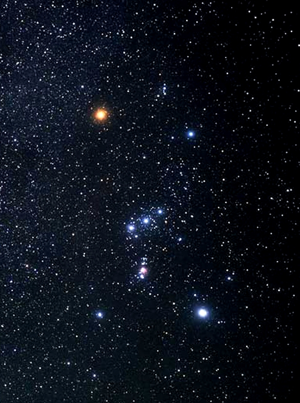
Fig. 1. The constellation of Orion (‘The Hunter’) in the night sky (east is to the left; north to the top).

Fig. 1. The constellation of Orion (‘The Hunter’) in the night sky (east is to the left; north to the top).
(1) Astronomical Nomenclature
Since ancient times the stars have been grouped together in constellations (“stars together”; Fig. 1). These star groups were given names reflecting the mythology of the time (Fig. 2), although today they have rigidly defined boundaries (Fig. 3). Some of the brightest stars were given individual names, which many still retain (e.g. Sirius, Polaris, Algol, Betelgeuse, etc).
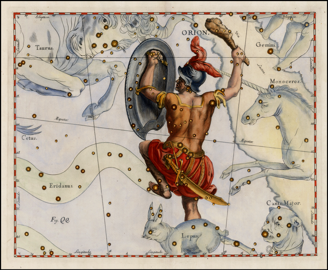
Fig. 2. Orion from a 17th Century map by Hevelius (NB. east and west are reversed in this map relative to what you see on the sky).

Fig. 2. Orion from a 17th Century map by Hevelius (NB. east and west are reversed in this map relative to what you see on the sky).
In 1603 the German astronomer Johann Bayer introduced the practice of giving Greek letters to the stars within constellations, generally in order of decreasing brightness (α, β, γ, ....). Thus Sirius, the brightest star in the constellation Canis Majoris (the ‘Big Dog’) is also known as α Canis Majoris (more usually abbreviated to α CMa), etc. Not all of Bayer’s rankings have been applied consistently, and since his time more careful measurements have shown that some stars are out of order (thus Rigel, β Ori, is actually a little brighter than Betelgeuse, α Ori), but Bayer’s classifications still give a good general guide to a star’s relative brightness (Fig. 3).
Only bright, naked eye, stars can be classified in this way. After telescopes began to be used (in 1609) it became possible to see vastly more stars, which were identified by giving each star a number in a catalogue. One of the first was due to the first English Astronomer Royal, John Flamsteed, who numbered stars sequentially from west to east within each constellation. Some of Flamsteed’s numbers are still in use (and some can be seen in Fig. 3).
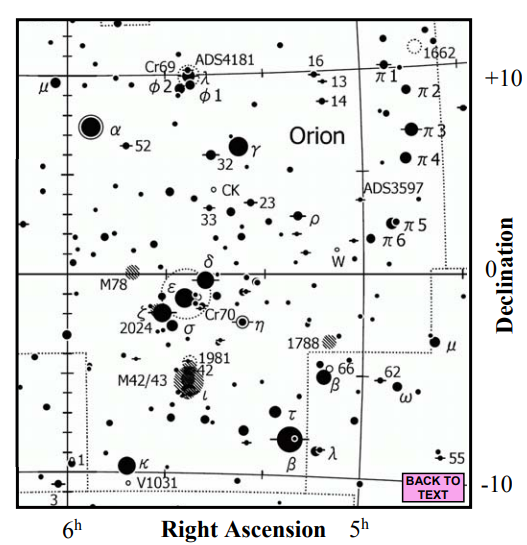
Fig. 3. A page from a modern star atlas showing the constellation of Orion. The defined boundary of the constellation is shown by dotted lines. Both Bayer letters and Flamsteed numbers are indicated. Objects marked with a capital M (from Messier’s catalogue) are not stars but nebulae; ‘Right Ascension’ and ‘Declination’ are the astronomical equivalent of longitude and latitude, respectively, and are described later in the lecture.

Fig. 3. A page from a modern star atlas showing the constellation of Orion. The defined boundary of the constellation is shown by dotted lines. Both Bayer letters and Flamsteed numbers are indicated. Objects marked with a capital M (from Messier’s catalogue) are not stars but nebulae; ‘Right Ascension’ and ‘Declination’ are the astronomical equivalent of longitude and latitude, respectively, and are described later in the lecture.
Today there are a large number of star catalogues, of which the largest lists over two and a half million stars (of which only about 5000 are visible to the naked eye). Such catalogues list the positions, magnitudes (i.e. brightness, see below), colour, and other information about each star. Fig. 4 shows a page from one such star catalogue.
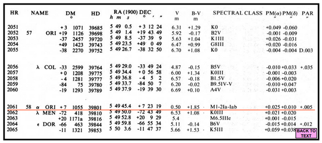
Fig. 4. A page from a modern star catalogue. HR, DM, and HD are numbers for the same star in different catalogues; RA and DEC are coordinates (see Fig. 3); V is the visual magnitude (brightness); (B-V) is a measure of a star’s colour, as is the ‘Spectral Class’; PM stands for ‘Proper Motion’ and is a measure of the star’s motion on the sky; PAR stands for ‘parallax’ and is a measure of the star’s distance. All these terms are explained in this or later lectures. Betelgeuse (α Ori; 58 Ori; HR 2061; HD 39801) is indicated by a red line.

Fig. 4. A page from a modern star catalogue. HR, DM, and HD are numbers for the same star in different catalogues; RA and DEC are coordinates (see Fig. 3); V is the visual magnitude (brightness); (B-V) is a measure of a star’s colour, as is the ‘Spectral Class’; PM stands for ‘Proper Motion’ and is a measure of the star’s motion on the sky; PAR stands for ‘parallax’ and is a measure of the star’s distance. All these terms are explained in this or later lectures. Betelgeuse (α Ori; 58 Ori; HR 2061; HD 39801) is indicated by a red line.
Note that, as the Galaxy is estimated to contain about 2×10¹¹ stars, only a very small fraction (about one in a hundred thousand) have ever been catalogued.
In addition to stars there are a variety of other astronomical objects visible in the night sky. These include objects in our own Solar System (such as planets, asteroids and comets), and more distant clouds of gas and dust (‘nebulae’) and external galaxies. As for the stars, the most prominent non-stellar objects have their own proper names (e.g. the Orion Nebula, visible in Fig. 1), but most are identified by numbers in specialist catalogues. Two of the most used is thee Messier Catalogue (a catalogue of 110 ‘fuzzy’ nebulae and star clusters produced by the French astronomer Charles Messier in 1771), and the larger ‘New General Catalogue of Nebulae and Clusters of Stars’ (published in 1888, initially with about 7800 objects but since expanded). Objects in the former catalogue are identified by a letter M, and in the latter by NGC; for example, the Orion Nebula is also known as M42 and NGC 1976 (see Fig. 3).
(2) Stellar Magnitudes
One of the most important pieces of information to be entered into a star catalogue is the brightness of a star on the sky, this is called its magnitude (more strictly its apparent magnitude, as described below). The concept of stellar magnitudes was introduced by the Greek astronomer Hipparchus (c.160-125 BC), who divided the visible stars into six magnitude bands, with 1 being the brightest and 6 the faintest (just visible to the unaided eye). Note that, in this scheme, brighter stars are said to have a smaller magnitude.
In the 18th century, William Herschel noted that we receive about a hundred times more light from a 1st magnitude star as from a 6th magnitude star. In 1856 this was verified by Norman Pogson and the magnitude scale was quantified so that a difference of 1 magnitude corresponds to a factor of 2.512 in brightness (as there are 5 magnitudes bands between magnitudes 1 and 6, and 2.512× 2.512× 2.512× 2.512× 2.512 = 100).
Thus, to two significant figures, a 2nd magnitude star is 2.5 times fainter than a 1st magnitude star, and 2.5 times brighter than a 3rd magnitude star; etc). When the system was first quantified, 1st magnitude was defined to be the average magnitude of the 20 brightest stars in the sky. As a result, in order to assign magnitudes to the very brightest stars in the sky, it was necessary to introduce the concept of ‘zero-magnitude’ (and, for the two brightest stars, negative magnitudes!).
Table 1 shows the relative magnitudes of some bright stars, compared with the observational limits of large telescopes.
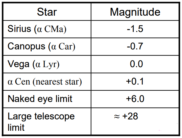
Table 1. Some representative stellar magnitudes compared with the detection limits of large telescopes (note that the latter actually depends on the length of time for which a given star is observed).

Table 1. Some representative stellar magnitudes compared with the detection limits of large telescopes (note that the latter actually depends on the length of time for which a given star is observed).
Note that a 28th magnitude star is (2.51)^28 = 1.5×10¹¹ times fainter than a star of magnitude zero.
These magnitudes are called “apparent magnitudes” because they describe how bright stars appear to be on the sky. The apparent magnitude of a star depends on three factors:
(a) The intrinsic brightness of the star;
(b) The distance of the star; and
(c) The extent to which a star’s light is dimmed by intervening clouds of gas and dust.
(3) Astronomical Coordinates
In order to locate objects on the sky, and to enter their positions into catalogues, it is necessary to give them coordinates, just as positions on the Earth’s surface can be specified in terms of their latitude and longitude. The most widely used astronomical the coordinate system is the equatorial coordinate system, based on a projection of the Earth’s equator on to the sky.
Like latitude and longitude on the Earth’s surface, the equatorial coordinate system specifies positions on the sky in a north-south direction, which astronomers call declination (Dec; δ), and an east-west direction, which astronomers call right ascension (RA; α).
Declination is just the angle to an astronomical object measured (in degrees) north (+) or south (–) of the Earth’s equator projected on to the sky (Fig. 5). The circle on the sky produced by extending the Earth’s equator like this is called the celestial equator, which therefore has a declination of zero degrees by definition.
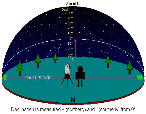
Fig. 5. Definition of declination.

Fig. 5. Definition of declination.
Right ascension is measured east-west, like longitude. However, as the RA of an astronomical object does not change as the Earth rotates, this coordinate must be measured from some fixed point on the sky (rather than a point fixed on the Earth, like the Greenwich meridian). The point chosen for this is the position of the Sun at the spring (or vernal) equinox (21 March), when the Sun is on the celestial equator. The location of the Sun at this time defines a point on the celestial equator which is fixed relative to the stars. Right ascension is measured eastwards along the equator from this point (Fig. 6).
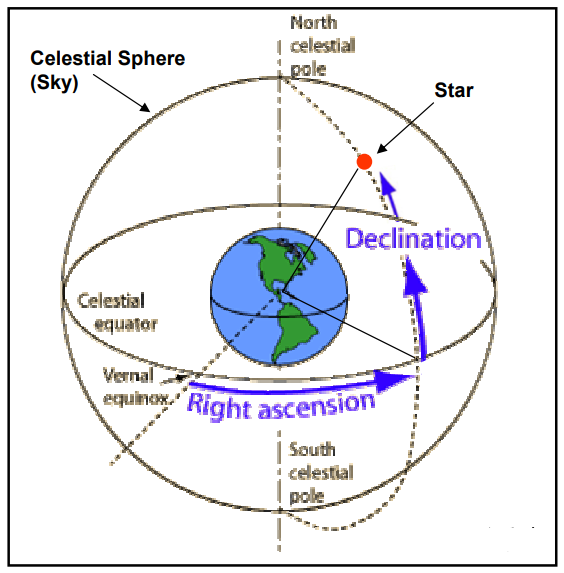
Fig. 6. The celestial sphere, showing the definition of right ascension and declination. The point marked ‘vernal equinox’ is the position of the Sun on the sky at the spring equinox (21 March).

Fig. 6. The celestial sphere, showing the definition of right ascension and declination. The point marked ‘vernal equinox’ is the position of the Sun on the sky at the spring equinox (21 March).
Right ascension, like declination, could be measured in degrees. However, because (until very recently) all astronomical observations have been taken from the surface of the rotating Earth, it has been found to be convenient to measure RA in units of time (i.e. hours, minutes and seconds). Because the Earth rotates once in 24 hours, one hour of right ascension corresponds to an angle of 15 degrees (since 360 ÷ 24 = 15). Thus, with this coordinate system, the positions of astronomical objects can be drawn on maps of the sky graduated in RA and Dec (see Fig. 3), and the coordinates can be entered into star catalogues (Fig. 4).
There is just one other minor complication, because of the effect of the Sun’s gravity on the spinning Earth, the Earth’s rotation axis does not remain fixed in space but processes about a line that is perpendicular to the plane of its orbit (the ecliptic plane), with a period of about 26,000 years (see Fig. 7). Thus, the vernal equinox is not absolutely fixed on the sky, but moves westwards at a rate of about 1 degree every 70 years (which therefore causes the RA of objects to increase at the same rate). Similarly, the celestial equator also moves with respect to the stars (Fig. 7). As a consequence star maps and catalogues always specify the date (or epoch) of the coordinates specified (e.g. 1900 for the example shown in Fig. 4).
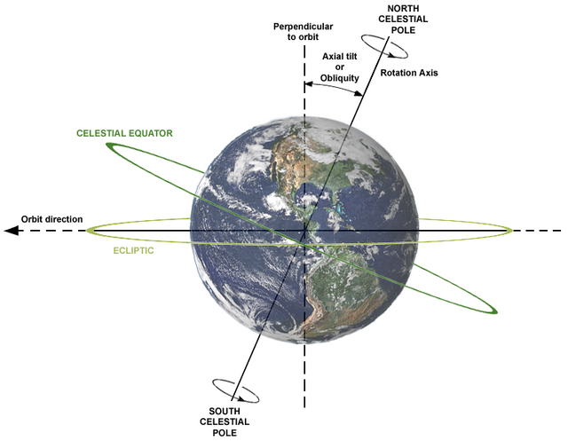
Fig. 7. Diagram showing the relationship between the Earth’s rotation axis and the ecliptic plane. The rotation axis precesses about the perpendicular to the ecliptic with a period of about 26,000 years, which must be allowed for when specifying equatorial coordinates.

Fig. 7. Diagram showing the relationship between the Earth’s rotation axis and the ecliptic plane. The rotation axis precesses about the perpendicular to the ecliptic with a period of about 26,000 years, which must be allowed for when specifying equatorial coordinates.
There are other coordinate systems in use in astronomy. For example, ecliptic coordinates are defined relative to the ecliptic plane (and are specified as ecliptic latitudes and longitudes), and galactic coordinates are measured relative to the galactic plane and the direction of the galactic centre (galactic latitudes and longitudes), but these need not concern us further here.
(4) Some other observational properties of stars
(4.1) Proper Motion
Stars are moving in space, typically with velocities of tens of km/s. These motions are mostly random, and superimposed on larger orbital velocities about the centre of the galaxy. None of these motions are large enough to be perceptible on the night sky in a human lifetime, but they can be measured by comparing photographs of the same area of the sky several years apart. This change in position is known as a star’s proper motion, and is expressed in terms of the annual change in right ascension and declination (see columns labelled ‘PM’ in Fig. 4). For the nearer stars, proper motion amounts to a few arc-seconds per year (where one arc-second = 1/3600 of a degree), but for most stars is much less. Note that, the Sun’s own motion through space also contributes to the observed proper motion of the stars, in addition to their own intrinsic motions.
(4.2) Double stars
When the telescope was first applied to astronomy it was noticed that many stars are double. A small fraction of these are chance alignments of closer and more distant stars (Fig. 8a). However, most double stars are true binary systems, where the two stars are physically orbiting each other (Fig. 8b).
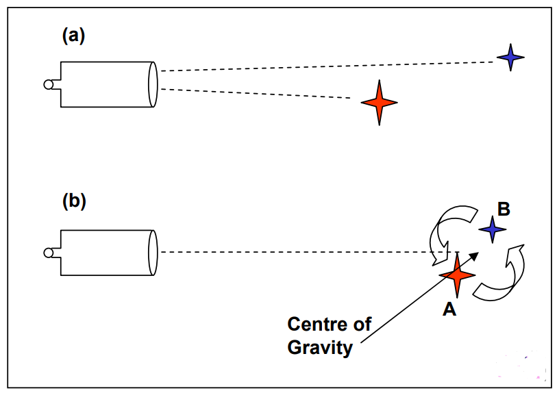
Fig. 8. Double stars. (a) A chance alignment on the sky. (b) Two stars gravitationally bound together and orbiting their common centre of gravity.

Fig. 8. Double stars. (a) A chance alignment on the sky. (b) Two stars gravitationally bound together and orbiting their common centre of gravity.
The brighter of the two stars within a binary system is generally labelled ‘A’ and the weaker ‘B’. Thus we can talk of Sirius A and Sirius B, etc. Triple star systems, and even larger multiplicities are known (with components then labelled, A, B, C., etc).
(4.3) Variable stars
Many stars are observed to be variable in their brightness, often by several magnitudes over periods of a few to many days (Fig. 9).
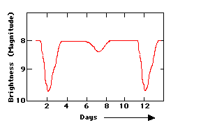
Fig. 9. Example of a light curve of a variable star.

Fig. 9. Example of a light curve of a variable star.
There are two main types of variable stars:
(a) Intrinsic variable stars, where the star itself changes its light output. There can be various reasons for this, including:
-• Pulsating stars
-• Flare stars
-• Star spots
(b) Eclipsing variable stars, where a binary star system is aligned such that one star passes in front of the other as seen from Earth.
Sources
Fig 1: http://www.constellation-guide.com/constellation-list/orion-constellation/
Fig 2: https://www.raremaps.com/gallery/detail/30201/Orion_Stars_heightened_in_gold/Hevelius.html
Fig 3:
Fig 5: http://calgary.rasc.ca/radecl.htm
Fig 6: http://hyperphysics.phy-astr.gsu.edu/hbase/eclip.html
Fig 7:
Fig 8: Birkbeck course material from Foundations of Astronomy
Fig 9: https://imagine.gsfc.nasa.gov/science/toolbox/timing1.html
Course: Birkbeck http://www.bbk.ac.uk/study/2018/undergraduate/programmes/UUBSPSAS_C