Training a Neural Network - A Numerical Example
Abstract
Neural networks are models used to approximate a discriminative function for classification in a supervised learning fashion. You have a bunch of input in the form of n-dimensional numerical vectors that represent features of certain entities you'd like to teach the network to classify (example 1000 emails classified as spam and 1000 emails classified non-spam). This paper takes a look at a quantitative approach in training a neural network given actual numerical examples. This will allow the student/practitioner to understand the fundamentals of the training process namely feed forward and backpropagation. The paper is intended to be light in concept with specific examples for people getting into machine learning with neural networks.
Introduction
Neural networks are biologically inspired computational models that attempts to solve classification problems. It is composed on neurons which holds and processes values in the network. You can think of these values as signal strengths that aim to mimic how chemical reactions occur in the brain. The higher the value, the stronger the signal. In biology, neurons transmit and receive signals to and from other neurons by means of dendrites. These propagations are modelled in the neural network by means of weight values. Since a neuron may receive values from more than one neuron, it accounts all the weights connected to it before attempting to fire a signal thus simulating how we "react" to certain stimuli. Training the neural network roughly means looking for the optimal values for these weights based on what we already know in order for the model to properly "react" to a certain input.
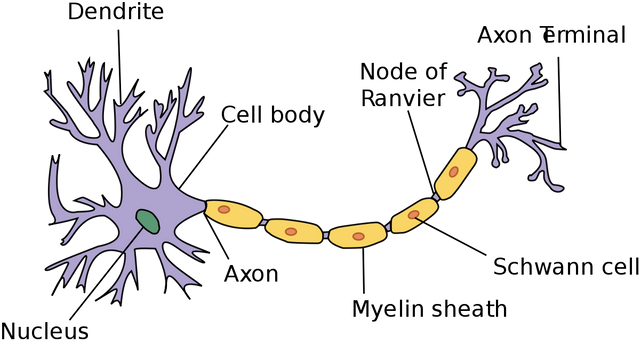
(Image taken from Wikipedia)
There are typically 3 layers in a classical neural network - input layer, hidden layer/s and output layer. These layers are connected to one another via neurons' weights in an adjacent manner. This means that a layer can only be connected to at most two adjacent layers. The input layer will always be the leftmost layer, the output layer will always be the rightmost layer while everything in between will be hidden layers. The following example is an illustration of the classical neural network:
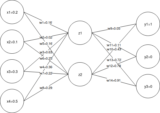
The image above will be the basis for the numeric computations in the following sections. But first, let's talk about the different components of the neural network.
Input Layer
The input layer contains neurons that represent the input values or what the network initially receives from the real world. These values are features that represent a classification/label that we'd like to recognize. In the mathematical model f(x) = y, this would be the x as an n-dimensional vector. For example, if we'd like to tell the neural network that we're looking at an image of a face represented by a matrix of pixel values, and suppose the size of the image is 32 x 32 pixels, the input layer would have a total of 1024 neurons each one corresponding to a pixel value. We refer to this vector as a feature vector.
Hidden Layer/s
From the input layer, information is passed to a hidden layer which contains neurons that processes signals it receives from the its adjacent layer/s (either from the left or from the right). A neural network can have more than one hidden layer. Neurons in the hidden layer are often denoted as z_i which we refer to as latent variables.
Output Layer
The output layer contains neurons that represent the output of the network or the result/reaction of the network after receiving and processing the input (from input layer to hidden layer then finally to the output layer). The easiest way to model neurons in the output layer is to treat each one (neuron) as a classification/label that the network is trying to recognize with a value ranging from 0 to 1. The closer the value to 1 for an output neuron, the closer it is to thinking that it is that classification or label for a given input x. For example, let's say we're trying to learn how to diffirentiate cats from dogs from any other animal. The set of possible outputs (cat, dog or others) can be represented by:
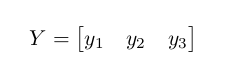
where y_1 represents the label cat, y_2 dog and y_3 others. A cat then for a neural network would look like $f(x) = \begin{bmatrix} 1 & 0 & 0 \end{bmatrix}$, a dog would be f(x) = [0, 1, 0] and finally any other animal f(x) = [0, 0, 1 ].
Training
To train a neural network means to optimize the set of weights (connections between neurons) in such a way that when we give it a feature vector representing a cat, the output should be close to f(x) = [1, 0, 0]. In order to do this, at the beginning of training, the weights are randomly initialized. We then feed it a feature vector relating to cat and see what the Y value is --- how close did the network get to the actual answer. This closeness value can be measured by a loss function. A higher value for this function means that the network yielded a higher error while smaller value means that the network is getting pretty close to recognizing what the input is. We will use this error/closeness value to adjust the weights accordingly. The first step in this entire training process is called feed forward.
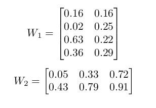
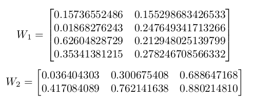
For the rest of the discussion, we will be referring to following figure for the initial weights:
Feed Forward
The feed forward process can be thought of the movement of information from the input layer in the form of the feature vector's values to the first hidden layer and finally making the guess (classification) in the output layer. Given two consecutive layers, information is passed from the left layer to the right layer by performing a matrix multiplication operation between the left layer's neurons and the weight matrix between the left and right layer. The resulting matrix should have the same size as the neurons in the right layer (1 row with n columns where n is the size of the neurons in the right layer). Let's take the following illustration:
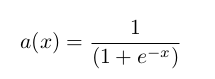
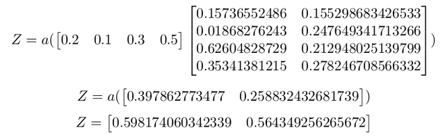
We're trying to solve for the values of Z by matrix multiplying X with W_1. The result will then be passed to an activation function such as the sigmoid function given by:
Mathematically, we can then represent information flow from X to Z:

Numerically we have the following:

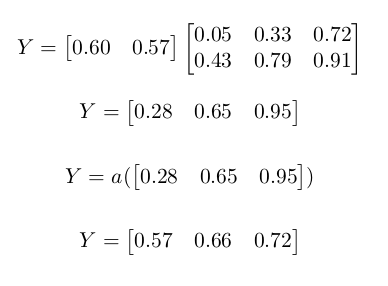
Using the same approach, we feed forward $Z$'s values towards $Y$ by matrix multiplying it with $W_{2}$.
Mathematically:
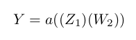
Numerically:
Loss Function
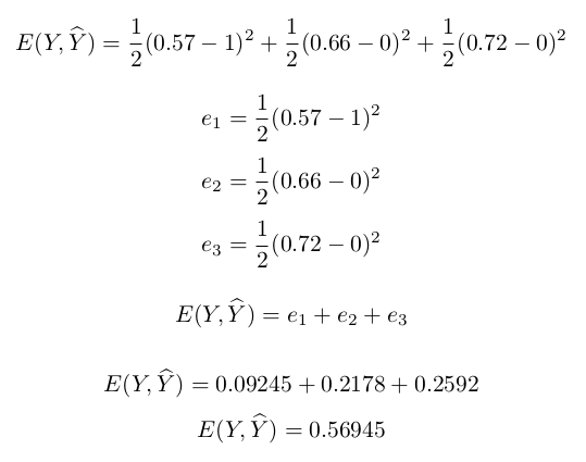
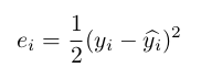
The loss function determines how far (or close) the guess of the network (Y) to the actual classification value (Y^). Remember that we want to teach the network how to recognize a certain classification by adjusting the its weights. The amount of adjustment we do will largely depend on the value given by the loss function. For this paper, we will be using a very simple loss function:

In the case of our example, Y^=[1, 0, 0], the value of our loss function will be computed as:
Back Propagation
Once we get the error value from the loss function, we can use this value to determine how much change we would apply to the weights to minimize this error value. This is done by a process called back propagation which takes the individual error values and cascades it from the output layer to the input layer seeing how much damage the weight values contributed to the overall error. Integral to this process is to solve for gradients. These gradients are approximation of derivatives. As with derivatives, gradient values dictate the direction of the error function of the network. If we know these values, we can roughly determine how to adjust our weights to minimize the error. To simplify things, since weight values drive the error value, we'd like to determine the gradient values for each neuron (since weights are attached to neurons) starting from the output layer (thus backward propagation) to give us the delta weights or how much magnitude should we adjust the original weights to lower the error. Numerically, this means that the size of our gradient vector will be the same size of neurons in a given layer.
For a more specific example, we'll break down this process into two major operations. The first part will perform back propagation starting from the output to the last hidden layer. And the second part will be from the last hidden layer down to the input layer. Similar to feed forward, we will be computing values with 3 inputs -- 2 layers and the weight matrix in between them. For each pair of layers, the gradient values to be computed for the right layer.
BP from Output to Last Hidden Layer
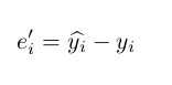
To start off, we compute the gradients for the right layer in this part of BP which in this case is the output layer (Y). Gradients are computed by taking the product of the first derivatives of equations used in the model. Take the loss function for each y_i for instance:
The first derivative e'_i for the loss function would be:
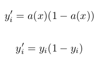
We also take the derivative for the neurons in the right layer (output layer in this case) which we will refer to as Y'. The activation function we used was:

The derivative a given output <code>y'_i</code> would approximately be:
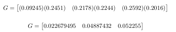
Given these derivatives, we can then compute for our gradients G_h (with a one to one correspondence to the right layer / output layer in this case). We can do this by using the following equation:
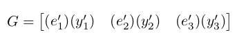
Plugging in the necessary values we have:
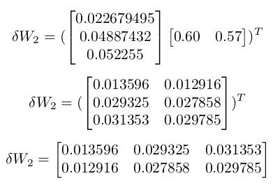
Once we have the gradient values, we can use these to compute for the the change in weight dW_2 which will subtract from the original weights to get the updated weights W^_2 (we're at index 2 because again we're moving from the last layer down to the input layer). At this part of the process, delta weights can be computed by multiplying the transpose of our gradients G with the output of the left layer -- in this case Z. We then transpose the result to have the same shape as W_2.

Plugging in the values we have:
Finally we can update the weights from Z to Y:

BP from Last Hidden Layer
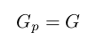
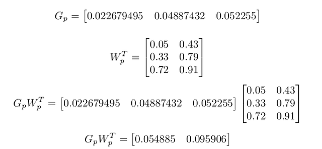
Computing the gradients and updated weights from the last hidden layer $Z$ down to the input layer $X$ is a bit different but generally follows the same process. Probably the major difference in this step of back propagation is to apply the gradients computed in the last operation (gradients corresponding to $Y$) as part of the computation. We shall refer to this as $G_{p}$ where:
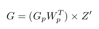
We then have to solve for a new $G$ which corresponds to the gradients of the right layer in this operation ($Z$). Aside from taking the previous operation's gradients, we have to also account for the old weights in the previous operation ($W_{2}$). We then matrix multiply $G_{p}$ with with the transpose of $W_{2}$ to give us the same shape as the right layer $Z$. This result will then be multiplied element-wise with the derivatives of $Z$ -- $Z'$. The operation would then be as follows:
Let's solve for the derivatives $Z'$ first using the same derivative equation as $Y'$:

Next we solve for $G_{p}W_{p}^T$:
Finally putting them all together to solve for $G = (G_{p}W_{p}^T) \times Z'$:

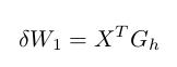
We can then extract the delta weights $\delta{W_{1}}$ using the following:
Plugging in the values we have:

If you have a deeper neural network, then we can apply the equations above to the next consecutive layers.
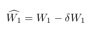
Now we can update $W_{1}$ to $\widehat{W_{1}}$ accordingly by subtracting $\delta{W_{1}}$ from it similar to what we did with $\widehat{W_{2}}$:
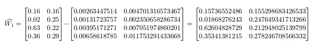
We now have the following updated weights for our network:
To test if we have indeed trained the network, we'll use the same input and perform a feed forward using the updated weights. This can be mathematically expressed:

Plugging in the values we have:


Finally we use the \textbf{loss function} to see if the network has improved (lower total error will incidcate improvement):
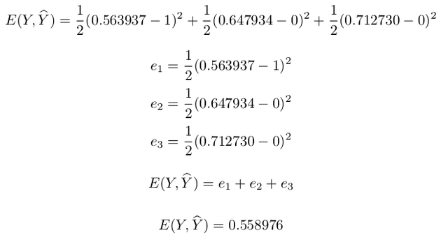
We now have $E(Y, \widehat{Y})=0.558976$ which is less than the initial error of $E(Y, \widehat{Y})=0.56945$.
Summary
This paper shows a numeric example on how we can train a classical fully connected neural network. "Training" a neural network refers to optimizing its weights to reduce the value of the \textbf{loss function} given a target $\widehat{Y}$. In this case, we used an optimization process called back propagation which takes the derivatives of the error values to propagates it to compute for gradients that indicates what direction the weights should move in order to minimize the error.
Congratulations @ralampay! You have completed some achievement on Steemit and have been rewarded with new badge(s) :
Click on any badge to view your own Board of Honor on SteemitBoard.
For more information about SteemitBoard, click here
If you no longer want to receive notifications, reply to this comment with the word
STOPCome and learn how AI processes images :)