Tutorial on Numerical Methods for Fiber Optics Gain Simulator by Using Python #Tutorial-7
What Will I Learn?
This tutorial covers the topics on scientific calculations such as integration, derivatives and interpolation by using scipy.integrate, scipy.misc and scipy.interpolate packages. Before continuing the previous tutorial which is about Fiber Optics Gain Simulator, we need to learn these calculations.
- You will learn integration by using scipy.integrate package.
- You will learn derivatives by using scipy.misc package.
- You will learn interpolation by using scipy.interpolate package.
Requirements
- Windows 8 or higher.
- Python 3.6.4.
- PyCharm Community Edition 2017.3.4 x64.
- Importing numpy, scipy, matplotlib packages
Difficulty
This tutorial has an indermadiate level.
Tutorial Contents
First of all, you need to import numpy, scipy, matplotlib, packages for this tutorial. To import these packages you can check our previous tutorials such as here. After importing the packages we need to call the packages which will be used in the program such as:
import numpy as importing
from scipy.integrate import *
from scipy.interpolate import interp1d
from scipy.misc import derivative
import matplotlib.pyplot as plotting
Let's start with integration. For numerical calculations, there are lots of types of interpretations of the integral such as Riemann–Darboux's integration, Lebesgue integration, trapezoidal and also quad one. This tutorial wil cover darboux, trapezoidal and quad integration and we will see the difference of these two integration types.
First of let's create a function such as:
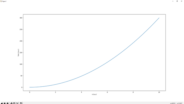
func=lambda x:3*x**2
x=importing.linspace(0,10,1000)
plotting.plot(x, func(x))
plotting.xlabel("x (a.u.)")
plotting.ylabel("func (a.u.)")
plotting.show()
This is the graph of 3x2 function for x between 0 and 10:
Let's write a code for numerical solution for darboux, trapezoidal methods such as:
func=lambda x:3*x**2

limitD=0
limitH=10
n=1000

hDarboux=(limitH-limitD)/n
hTrapezoidal=(limitH-limitD)/n

Eqn1=(func(limitD)+func(limitH))
for i in range(1,n):
    Eqn1=func(limitD+i*hDarboux)+Eqn1
    #Eqn+=f(a+i*h)
IntegralSolutionDarboux=hDarboux*Eqn1

Eqn2=0.5*(func(limitD)+func(limitH))
for i in range(1,n):
    Eqn2=func(limitD+i*hTrapezoidal)+Eqn2
    #Eqn2+=f(a+i*h)
IntegralSolutionTrapezoidal=hTrapezoidal*Eqn2

print(IntegralSolutionDarboux)
print(IntegralSolutionTrapezoidal)
The results are:
1001.5005000000004--IntegralSolutionDarboux
1000.0005000000008--IntegralSolutionTrapezoidal
As you see that if you divide your graph into 1000 elements then the result has a some errors. For Darboux method the error is almost 0.15% and for trapezoidal method, the error is almost 0.00005%. However, quad method is the best for integration method which will give you an error below 10-10%. Let's check:
print(quad(func,limitD,limitH))
The result:
(1000.0000000000001, 1.1102230246251567e-11)
As you see there are result. First element is the result and the second one is the error. You can take these data for different variables such as:
result, error=(quad(func,limitD,limitH))
print(result)
print(error)
For quad method you will write like this, quad(function, first limit, second limit).
As a result for trapezoidal or Darboux methods will be good for imported data. Because for imported data you cannot define your difference of the x element for f(x). But for just calculations you can use quad subpackage easily.
Let's move on derivatives. First of all, create a function:
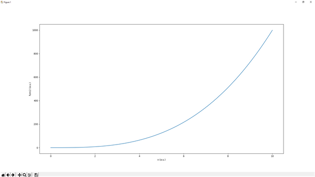
func2=lambda x:x**3
x=importing.linspace(0,10,1000)
plotting.plot(x,func2(x))
plotting.xlabel("x (a.u.)")
plotting.ylabel("func2 (a.u.)")
plotting.show()
This is the graph of x3 function for x between 0 and 10:
Then let's take the first derivative of this function such as:
print(derivative(func2,10,dx=1e-10))
To see on graph:
func2=lambda x:x**3

a=[]
print(derivative(func2,10,dx=1e-10))
x=importing.linspace(0,10,1000)
for i in range(1,len(x)):
    a.append(int(derivative(func2,x[i],dx=1e-10)))
plotting.plot(x,func2(x),label="func2")
plotting.plot(x[0:999],a,label="derivative of func2")
plotting.xlabel("x (a.u.)")
plotting.legend()
plotting.show()
The result:
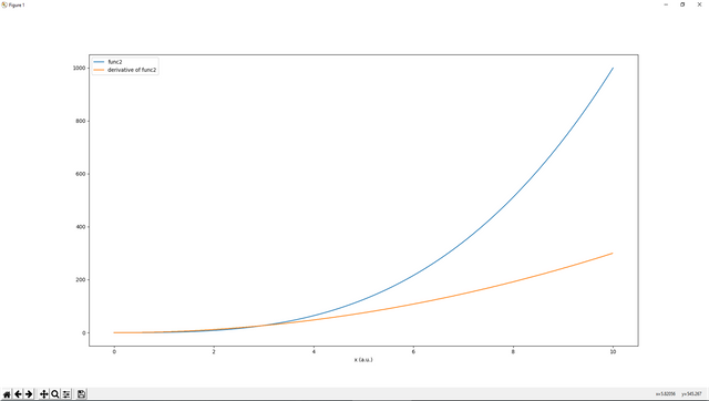
As you see that the derivative method is used like this, derivative(function, x=, dx=error).
Let's move on interpolation. In this tutorial we will examine three different interpolation method such as linear, quadratic and cubic such as:
x=importing.linspace(0,10,10)
y=10*importing.random.randn(10)
plotting.plot(x,y,'bo',label='Real Data')

xLinear=importing.linspace(0,10,100)
yLinear=interp1d(x,y,kind='linear')
plotting.plot(xLinear,yLinear(xLinear),'r',label='Linear Interpolation')

xQuad=importing.linspace(0,10,100)
yQuad=interp1d(x,y,kind='quadratic')
plotting.plot(xQuad,yQuad(xQuad),'k--',label='Quadratic Interpolation')

xCubic=importing.linspace(0,10,100)
yCubic=interp1d(x,y,kind='cubic')
plotting.plot(xCubic,yCubic(xCubic),'g',label='Cubic Interpolation')
plotting.legend()
plotting.show()
The result is :
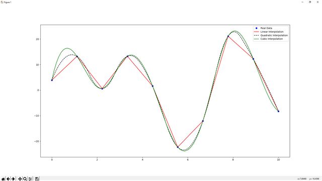
The usage is like this. For interp1d method we need to create a new array for interpolation (higher number of array means higher resolution). Then we need to make a interpolation for real data such as yMethod=interp1d(real x data, real y data, kind='method'), method can be 'linear', 'quadratic' or 'cubic'. yMethod is a just a function and we can define our variables such as yMethod(new x data). Then we have interpolated data.
In this tutorail we learnt how to take integration, derivatives and interpolation and gave some graphical examples on these topics by using matplotlib.pyplot package.
Curriculum
Here is the list of related tutorials we have already shared on @utopian-io community.
- Tutorial on Fiber Optics Gain Simulator by Using Python #Tutorial-6
- Tutorial on Plotting by Using matplotlib Package and Giving an Example of FFT Analysis in Python #Tutorial-5
- Tutorial on GUI (continues) and Example of Web Crawler by combining PyQt5 and BeautifulSoup package in Python #Tutorial-4
- Tutorial on GUI and Example of Simple Addition Calculator by using PyQt5 package in Python #Tutorial-3
- Creating Package and Subpackage in Python #Tutorial-2
- Example of Steemit Analysis by Using Python #Tutorial-1
Posted on Utopian.io - Rewarding Open Source Contributors
Thanks for the contribution.
Need help? Write a ticket on https://support.utopian.io.
Chat with us on Discord.
[utopian-moderator]
Hey @deathwing, I just gave you a tip for your hard work on moderation. Upvote this comment to support the utopian moderators and increase your future rewards!
Congratulations! This post has been upvoted from the communal account, @minnowsupport, by onderakcaalan from the Minnow Support Project. It's a witness project run by aggroed, ausbitbank, teamsteem, theprophet0, someguy123, neoxian, followbtcnews, and netuoso. The goal is to help Steemit grow by supporting Minnows. Please find us at the Peace, Abundance, and Liberty Network (PALnet) Discord Channel. It's a completely public and open space to all members of the Steemit community who voluntarily choose to be there.
If you would like to delegate to the Minnow Support Project you can do so by clicking on the following links: 50SP, 100SP, 250SP, 500SP, 1000SP, 5000SP.
Be sure to leave at least 50SP undelegated on your account.
Hey @onderakcaalan! Thank you for the great work you've done!
We're already looking forward to your next contribution!
Fully Decentralized Rewards
We hope you will take the time to share your expertise and knowledge by rating contributions made by others on Utopian.io to help us reward the best contributions together.
Utopian Witness!
Vote for Utopian Witness! We are made of developers, system administrators, entrepreneurs, artists, content creators, thinkers. We embrace every nationality, mindset and belief.
Want to chat? Join us on Discord https://discord.me/utopian-io
Thanks to @utopian-io community...