Tutorial on Fiber Optics Gain Simulator by Using Python #Tutorial-6
What Will I Learn?
This tutorial covers the topics on Fiber Optics Gain Simulator which includes numpy for importing data from .txt files, matplotlib for graphs, scipy.fftpack for fft analysis and PyQt5 GUI packages. For this simulation there will be 3 or 4 tutorials. This is the first part of the simulation which includes Ytterbium and Erbium gain fibers' absorption and emission graphs and also creating some gaussian signal and its wavelength conversion. This tutorial will be interested in by @steemstem community due to some scientific calculations understanding the Fiber Optic Simulations. At the end of the tutorails, we will create a package about Fiber Optics Gain Simulator to make simulation how the input signal amplifies through the gain fibers.
- You will learn importing file from .txt files by using numpy package.
- You will learn creating some functions such as Gaussian and its fft analysis to get spectrum conversion by using scipy.fftpack package.
- You will learn how to use GUI window by using PyQt5 package.
- You will learn how to make a plots and also subplots by using matplotlib package.
Requirements
Write here a bullet list of the requirements for the user in order to follow this tutorial.
- Windows 8 or higher.
- Python 3.6.4.
- PyCharm Community Edition 2017.3.4 x64.
- Importing numpy, scipy.fftpack, matplotlib, PyQt5 and scipy packages
Difficulty
This tutorial has an indermadiate level.
Tutorial Contents
First of all, you need to import the numpy, scipy.fftpack, matplotlib, PyQt5 and scipy packages for this tutorial. To import these packages you can check our Tutorials such as here. After importing the packages we need to call the packages which will be used in the program such as:
import numpy as importing
import matplotlib.pyplot as plotting
from scipy.fftpack import fft
import sys
from PyQt5 import QtWidgets
from PyQt5.QtWidgets import QMainWindow, QWidget, QPushButton, QLineEdit,QInputDialog
As you see that we defined some modules for some packages such as importing, plotting etc. This is for easy usage. Because when you want to call the package you do not need to remember the name of the package and also you can create some abbreviations not to write long names. Also if you want to call some subpackages you can use from ... import ... codes then you can get rid of writing full package and subpackage.
To create a simple, easy and effective GUI by using PyQt5 package, you need to make a plan such that:
- You need to create a class to start the QWidgets subpackes inside the PyQt5 package.
class Main(QtWidgets.QWidget):
...
...
...
if __name__ == "__main__":
    main()
- Then to continue program until you stop the program or quit the window, you need to add a function at the end of the program.
def main():
   app = QtWidgets.QApplication(sys.argv)
   main = Main()
   main.show()

   sys.exit(app.exec_())
- You need to create a function which is explained in our previous tutorials such as
We used init() constructor method to call inherited class which helps us not to write in each line to call our inherited class. Just we need to write self. it will be enough. Actually, you can change the name of variable self. but when we search websites they always suggest of usage of this as self..[1]
    def __init__(self):
        QtWidgets.QWidget.__init__(self)
        self.initUI()
Now we can write our program inside initUI functions. As you see we are using ** self** variable inside our functions because we do not want to call them from a spesific variables. This is for GUI data and these data will be always prepared inside the window.
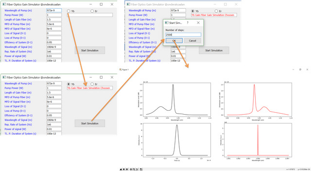
First of all, for our GUI we created our title, variables, buttons (push, radio), labels, lines such as:
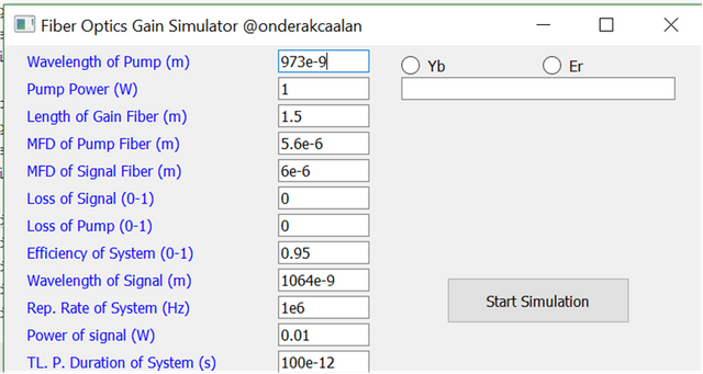
For each variables, we used QtWidgets.QLineEdit() method. Also you can move the line by using .move method and also define the boundaries of the label by using .resize method. If you want to give some initial variables you can set a text (it can be float, integer also string) and if you do not want to be changed this text by users you can define it as a read only by using .setReadOnly.
self.pumpWavelength = QtWidgets.QLineEdit(self)
        self.pumpWavelength.move(300, 5)
        self.pumpWavelength.setText("973e-9")
        #self.pumpWavelength.setReadOnly(True)
        self.pumpWavelength.resize(100, 25)
Also we want to give some name for these lines to understand which line means. To do that we used QtWidgets.QLabel methods. We want to emphasize these labels by changing color by using .setStyleSheet method.
self.pumpPower = QtWidgets.QLabel("Pump Power (W)", self)
        self.pumpPower.setStyleSheet("color:blue")
        self.pumpPower.move(25, 35)
        self.pumpPower.resize(200, 25)
If you want to use .setStyleSheet method effectively you can check this website.
setStyleSheet("color: blue;"
"background-color: yellow;"
"selection-color: yellow;"
"selection-background-color: blue;");[2]
Then we added some buttons to do some works on GUI. For example, we created two radio buttons to import some data from .txt files and kept those data to work such as:
getInfo2 = QtWidgets.QRadioButton("Yb", self)
        getInfo2.toggled.connect(self.Yb)
        getInfo2.move(435, 0)
        getInfo2.resize(150, 45)
As you see, here we defined a function getInfo2 and connected to self.Yb function by using .toggled.connect method (For different buttons you need to use different connection methods. We will show in this tutorial for push button also.). Because we want to call some data from a file when we push the button. If we do not push the button or if we push another button the data which we want to call will change such as:
    def Yb(self):
        Checked = self.sender()
        if Checked.isChecked():
            self.GainHeader.setText("Yb Gain Fiber Gain Simulation Choosen")
            self.pumpWavelength.setText("973e-9")
            self.signalMFD.setText("6e-6")
            self.signalWavelength.setText("1064e-9")
To work on self.Yb function we need to create a function. Then by using .self.sender() method we can keep a info about the button is clicked or not. Then by using if statement we can write some duties for this function. To check the situation we used .isChecked() method. For example, here, we want to write a line such as "Yb Gain Fiber Gain Simulation Choosen" by using .setText to use this sentence to call another function (we will explain later). Then we added some other duties also.
For push button we assigned a duty about starting the simulation. The main function is related to this button. To create this button we used QtWidgets.QPushButton method such as:
getInfo1 = QtWidgets.QPushButton("Start Simulation", self)
        getInfo1.move(485, 255)
        getInfo1.resize(200, 50)
        getInfo1.clicked.connect(self.getText)
Also we created a function for this button by using .clicked.connect method and the name of the function will be get #of steps data starts the simulator such as:
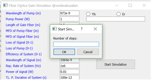
Inside this function we wrote our Fiber Optic Gain Simulator program. Here, we want to explain how to create the simulator and also plotting the data. This will be a little bit scientific also. If you do not want to read scientific parts you can skip that parts and read the methods parts.
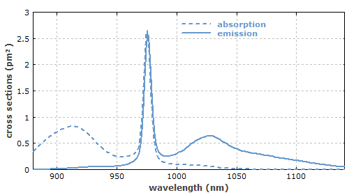
For optical gain fiber, first of all we need to create a absorption and emission spectrum ratesfor the gain fibers and we got these data from a scientific paper which is [Optics Letters]([ref. Opt. Lett. 33(19), 2221-2223]). If you check websites such as Yb (or Er) absorption and emission spectrum graphs you will find this graph. To get the data from a .txt file we used .loadtxt method inside numpy package. Maybe you remember from upside part we defined a GainHeader which is defined when we push Yb radio buttons. We used that radio button output and check the button name. If we push Yb button then:
            if self.GainHeader.text()=="Yb Gain Fiber Gain Simulation Choosen":
                xlam = importing.loadtxt('xlam.txt', unpack=True)  # wavelength range
                ya = importing.loadtxt('ya.txt', unpack=True)  # Ytterbium absorption data
                ye = importing.loadtxt('ye.txt', unpack=True)  # Ytterbium  emission data
If push Er button then:
            if self.GainHeader.text()=="Er Gain Fiber Gain Simulation Choosen":
                xlam = importing.loadtxt('xlam.txt', unpack=True)  # wavelength range
                ya = importing.loadtxt('ya.txt', unpack=True)  # Erbium absorption data
                ye = importing.loadtxt('ye.txt', unpack=True)  # Erbium emission data
Before creating our input signal (scientifically not program signal:D) we define our variables such as center wavelength, pump power, transform limited pulse duration etc. Each of them is getting from the window part by using .text method such as: For numpy package you need to define your variables as float (float()) or integer (int()) because sometimes numpy package change the variables and you took some errors.
c = 3e8  # Speed of light [m/s]
            h = 6.626e-34  # Planck constant [J.s]
            P_p = float(self.pumpPower.text())  # Pump power [W]

            L = float(self.lengthGain.text())  # Length [m]
            d_core = 4e-6  # Core diameter [m]
            mfd_pump = float(self.pumpMFD.text()) # Mode-field diameter for pump [m]
            mfd_signal = float(self.signalMFD.text())  # Mode-field diameter for signal [m]
            alpha_s = float(self.signalLoss.text())  # signal loss [m^-1]
            alpha_p = float(self.pumpLoss.text())  # pump loss [m^-1]
            ...
            ...
            eta = float(self.efficiency.text())  # efficiency coefficient [a.u.]
            t1 = 0.85e-3  # upper state life time [s]
            ...
            ...
To create our signal we need time and energy scale. To crate time scale we used .linspace method such as:
time = importing.linspace(-tres / 2, tres / 2 - 1, tres) * (T / 1.665 / t0) # Time axis [s]
Here, "tres" is "Total number of data points". As you see that, this method is used by .linspace(starting boundary, last boundary, # of data). Scientificly, we proportion to our time scale by gaussian scale which is (T / 1.665) where T is the trasnform limited pulse duration and 1.665 is a constant for gaussian scale. Also we divided the time sclae to "Number of data points corresponds to FWHM" to get exact value.
To create our E-field:
 E_p = (P_s / f_rep)  # Pulse energy [J]
            peak_s = E_p / (T / 1.665) / importing.sqrt(importing.pi)  # Peak power of the pulse [W]
 E = importing.sqrt(peak_s) * importing.exp((time * time) / (-2) / (T / 1.665) / (T / 1.665))  # Electric field array
First of we need to find our peak power of the pulse so we used pulse energy which can be found power/repetition rate of the system. Then by using peak power and time scale we can find electric field of the input signal. As you see that to use some mathematical expressions such as square root*, pi, exp, etc. we used numpy package. importing module is defined as importing numpy package which was eplained in the beginning of the tutorial.
Then we created frequency axis and wavelength axis such as:
fr = c / lambda_s + importing.linspace(-tres / 2 + 1, tres / 2, tres) * (t0 / T * 1.665) / (tres * 1.0) # Frequency axis [Hz]
lambd = c / fr  # Wavelength axis [m]
Then we need to shift our electric field array to zero so we used a shifthing part such as:
            if tres / 2 > 0:
                aux1 = (E[(int(m) - int(tres / 2)):int(m)])
                aux2 = ((E[0:(int(m) - int(tres / 2))]))
                field2 = [(aux1), (aux2)]
            a = field2[0]
            b = field2[1]

            for j in range(len(a)):
                c = a[j]
                E2.append(c)
            for j in range(len(b)):
                c = b[j]
                E2.append(c)
            E2 = E
            # shifting stops
Here, we could not find any method to convert two numpy.array into one array. There are lots of suggestions such as .concatenate or .hstack. However nothing worked so we created our method and convert our two array data to one array by using for loops. If you know how to it please contact us.
Here is the electric field of our input signal:
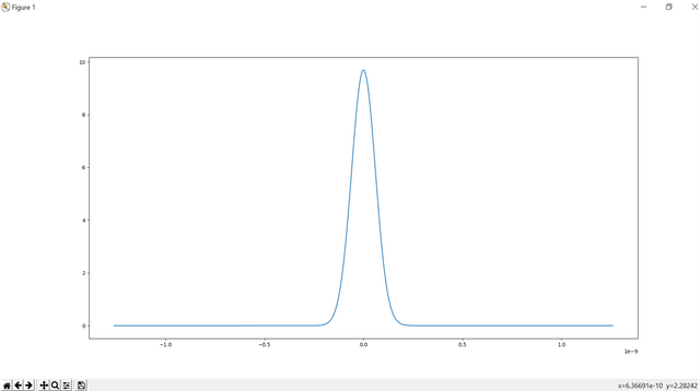
As you see that the pulse width is 100ps and the shape is gaussian.
Then we convert our electric field to spectrum domain such as:
# spectrum analysis starts
           Ef1 = fft(E)
            Ef = importing.linspace(0, 0, int(tres))
            for f in range(int(tres / 2)):
                freal = int(tres / 2 + f - 1)
                Ef[freal] = importing.abs(Ef1[f]) * importing.abs(Ef1[f])
            print(Ef)
            print(importing.linspace(int(tres / 2 + 1), int(tres - 1), int(tres - 1) - int(tres / 2 + 1) + 1))
            for f in importing.linspace(int(tres / 2 + 1), int(tres - 1), int(tres - 1) - int(tres / 2 + 1) + 1):
                freal = int(f) - int((tres / 2 + 1))
                Ef[freal] = importing.abs(Ef1[int(f)]) * importing.abs(Ef1[int(f)])
            print(Ef)
            Spect = 1.01678 * T * T / 1.665 / (t0 * t0) / (lambda_s * lambda_s) * 1e8 * importing.sqrt(
                importing.pi) * Ef
            # spectrum analysis finishes
If you know how to make fft analysis, you will easily understanfd this part. your half of data will be same with the other half. So you need to divide your data after fft part which is made by fft() method and then combine them as one of half will be reverse.
The result of the spectrum analysis is:
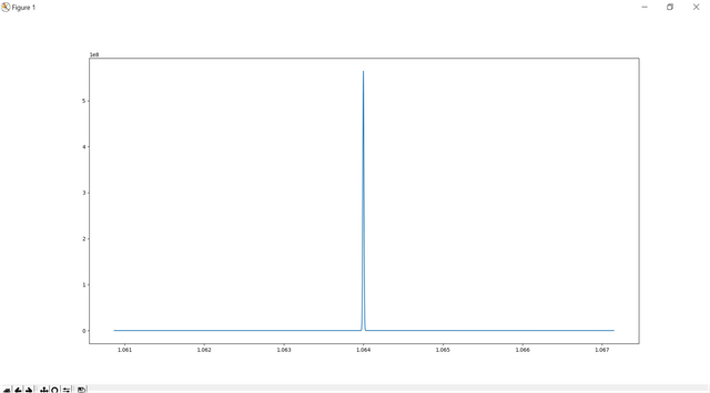
When we check linewidth we see that the linewidth is 0.015nm which is considerable with the transform limited pulse duration which is 100ps.
Then we used matplotlib package to see the results on graph as a subplot:
plotting.figure(1)
            plotting.subplot(221)
            plotting.plot(xlam * 1000000,ya, 'k')

            plotting.subplot(222)
            plotting.plot(xlam * 1000000,ye, 'r--')

            plotting.subplot(223)
            plotting.plot(time, E, 'k')

            plotting.subplot(224)
            plotting.plot(lambd * 1000000, Spect * f_rep, 'r--')
            plotting.show()
As you see if you want to create a subplot you can use.subplot method by defining the row and column and the number of place. For example here, we created 2x2 subplot and we placed our subplots inside this plot.
Here is the all code:
import numpy as importing
import matplotlib.pyplot as plotting
from scipy.fftpack import fft
import sys
from PyQt5 import QtWidgets
from PyQt5.QtWidgets import QMainWindow, QWidget, QPushButton, QLineEdit,QInputDialog
import re

class Main(QtWidgets.QWidget):

    def __init__(self):
        QtWidgets.QWidget.__init__(self)
        self.initUI()

    def initUI(self):

        self.setWindowTitle('Fiber Optics Gain Simulator @onderakcaalan')

        self.pumpWavelength = QtWidgets.QLabel("Wavelength of Pump (m)", self)
        self.pumpWavelength.setStyleSheet("color:blue")
        self.pumpWavelength.move(25, 5)
        self.pumpWavelength.resize(200, 25)

        self.pumpWavelength = QtWidgets.QLineEdit(self)
        self.pumpWavelength.move(300, 5)
        self.pumpWavelength.setText("973e-9")
        #self.pumpWavelength.setReadOnly(True)
        self.pumpWavelength.resize(100, 25)

        self.pumpPower = QtWidgets.QLabel("Pump Power (W)", self)
        self.pumpPower.setStyleSheet("color:blue")
        self.pumpPower.move(25, 35)
        self.pumpPower.resize(200, 25)

        self.pumpPower = QtWidgets.QLineEdit(self)
        self.pumpPower.move(300, 35)
        self.pumpPower.setText("1")
        #self.pumpPower.setReadOnly(True)
        self.pumpPower.resize(100, 25)

        self.lengthGain = QtWidgets.QLabel("Length of Gain Fiber (m)", self)
        self.lengthGain.setStyleSheet("color:blue")
        self.lengthGain.move(25, 65)
        self.lengthGain.resize(200, 25)

        self.lengthGain = QtWidgets.QLineEdit(self)
        self.lengthGain.move(300, 65)
        self.lengthGain.setText("1.5")
        #self.lengthGain.setReadOnly(True)
        self.lengthGain.resize(100, 25)

        self.pumpMFD = QtWidgets.QLabel("MFD of Pump Fiber (m)", self)
        self.pumpMFD.setStyleSheet("color:blue")
        self.pumpMFD.move(25, 95)
        self.pumpMFD.resize(200, 25)

        self.pumpMFD = QtWidgets.QLineEdit(self)
        self.pumpMFD.move(300, 95)
        self.pumpMFD.setText("5.6e-6")
        #self.pumpMFD.setReadOnly(True)
        self.pumpMFD.resize(100, 25)

        self.signalMFD = QtWidgets.QLabel("MFD of Signal Fiber (m)", self)
        self.signalMFD.setStyleSheet("color:blue")
        self.signalMFD.move(25, 125)
        self.signalMFD.resize(200, 25)

        self.signalMFD = QtWidgets.QLineEdit(self)
        self.signalMFD.move(300, 125)
        self.signalMFD.setText("6e-6")
        #self.signalMFD.setReadOnly(True)
        self.signalMFD.resize(100, 25)

        self.signalLoss = QtWidgets.QLabel("Loss of Signal (0-1)", self)
        self.signalLoss.setStyleSheet("color:blue")
        self.signalLoss.move(25, 155)
        self.signalLoss.resize(200, 25)

        self.signalLoss = QtWidgets.QLineEdit(self)
        self.signalLoss.move(300, 155)
        self.signalLoss.setText("0")
        #self.signalLoss.setReadOnly(True)
        self.signalLoss.resize(100, 25)

        self.pumpLoss = QtWidgets.QLabel("Loss of Pump (0-1)", self)
        self.pumpLoss.setStyleSheet("color:blue")
        self.pumpLoss.move(25, 185)
        self.pumpLoss.resize(200, 25)

        self.pumpLoss = QtWidgets.QLineEdit(self)
        self.pumpLoss.move(300, 185)
        self.pumpLoss.setText("0")
        #self.pumpLoss.setReadOnly(True)
        self.pumpLoss.resize(100, 25)

        self.efficiency = QtWidgets.QLabel("Efficiency of System (0-1)", self)
        self.efficiency.setStyleSheet("color:blue")
        self.efficiency.move(25, 215)
        self.efficiency.resize(200, 25)

        self.efficiency = QtWidgets.QLineEdit(self)
        self.efficiency.move(300, 215)
        self.efficiency.setText("0.95")
        #self.efficiency.setReadOnly(True)
        self.efficiency.resize(100, 25)

        self.signalWavelength = QtWidgets.QLabel("Wavelength of Signal (m)", self)
        self.signalWavelength.setStyleSheet("color:blue")
        self.signalWavelength.move(25, 245)
        self.signalWavelength.resize(200, 25)

        self.signalWavelength = QtWidgets.QLineEdit(self)
        self.signalWavelength.move(300, 245)
        self.signalWavelength.setText("1064e-9")
        #self.signalWavelength.setReadOnly(True)
        self.signalWavelength.resize(100, 25)

        self.repRate = QtWidgets.QLabel("Rep. Rate of System (Hz)", self)
        self.repRate.setStyleSheet("color:blue")
        self.repRate.move(25, 275)
        self.repRate.resize(200, 25)

        self.repRate = QtWidgets.QLineEdit(self)
        self.repRate.move(300, 275)
        self.repRate.setText("1e6")
        #self.repRate.setReadOnly(True)
        self.repRate.resize(100, 25)

        self.signalPower = QtWidgets.QLabel("Power of signal (W)", self)
        self.signalPower.setStyleSheet("color:blue")
        self.signalPower.move(25, 305)
        self.signalPower.resize(200, 25)

        self.signalPower = QtWidgets.QLineEdit(self)
        self.signalPower.move(300, 305)
        self.signalPower.setText("0.01")
        #self.signalPower.setReadOnly(True)
        self.signalPower.resize(100, 25)

        self.TLpulseDuration = QtWidgets.QLabel("TL. P. Duration of System (s)", self)
        self.TLpulseDuration.setStyleSheet("color:blue")
        self.TLpulseDuration.move(25, 335)
        self.TLpulseDuration.resize(250, 25)

        self.TLpulseDuration = QtWidgets.QLineEdit(self)
        self.TLpulseDuration.move(300, 335)
        self.TLpulseDuration.setText("100e-12")
        #self.TLpulseDuration.setReadOnly(True)
        self.TLpulseDuration.resize(100, 25)

        getInfo1 = QtWidgets.QPushButton("Start Simulation", self)
        getInfo1.move(485, 255)
        getInfo1.resize(200, 50)
        getInfo1.clicked.connect(self.getNumofSteps)

        getInfo2 = QtWidgets.QRadioButton("Yb", self)
        getInfo2.toggled.connect(self.Yb)
        getInfo2.move(435, 0)
        getInfo2.resize(150, 45)

        getInfo3 = QtWidgets.QRadioButton("Er", self)
        getInfo3.toggled.connect(self.Er)
        getInfo3.move(590, 0)
        getInfo3.resize(150, 45)

        self.GainHeader = QtWidgets.QLineEdit(self)
        self.GainHeader.move(435, 35)
        self.GainHeader.setReadOnly(True)
        self.GainHeader.setStyleSheet("color:red")
        self.GainHeader.resize(300, 25)

    def Yb(self):
        Checked = self.sender()
        if Checked.isChecked():
            self.GainHeader.setText("Yb Gain Fiber Gain Simulation Choosen")
            self.pumpWavelength.setText("973e-9")
            self.signalMFD.setText("6e-6")
            self.signalWavelength.setText("1064e-9")

    def Er(self):
        Checked = self.sender()
        if Checked.isChecked():
            self.GainHeader.setText("Er Gain Fiber Gain Simulation Choosen")
            self.pumpWavelength.setText("973e-9")
            self.signalMFD.setText("10e-6")
            self.signalWavelength.setText("1550e-9")

    def getNumofSteps(self):
        text, OKPressed = QInputDialog.getText(self, "Start Simulation", "Number of steps:", QLineEdit.Normal, "")
        if OKPressed and text != '':
            c = 3e8  # Speed of light [m/s]
            h = 6.626e-34  # Planck constant [J.s]
            P_p = float(self.pumpPower.text())  # Pump power [W]

            L = float(self.lengthGain.text())  # Length [m]
            d_core = 4e-6  # Core diameter [m]
            mfd_pump = float(self.pumpMFD.text()) # Mode-field diameter for pump [m]
            mfd_signal = float(self.signalMFD.text())  # Mode-field diameter for signal [m]
            alpha_s = float(self.signalLoss.text())  # signal loss [m^-1]
            alpha_p = float(self.pumpLoss.text())  # pump loss [m^-1]
            eta = float(self.efficiency.text())  # efficiency coefficient [a.u.]
            t1 = 0.85e-3  # upper state life time [s]

            Ntot = 9e25 / 2  # [ref. Opt. Lett. 33(19), 2221-2223]

            if self.GainHeader.text()=="Er Gain Fiber Gain Simulation Choosen":
                xlam = importing.loadtxt('xlam.txt', unpack=True)  # wavelength range
                ya = importing.loadtxt('ya.txt', unpack=True)  # Erbium absorption data
                ye = importing.loadtxt('ye.txt', unpack=True)  # Erbium emission data
            elif self.GainHeader.text()=="Yb Gain Fiber Gain Simulation Choosen":
                xlam = importing.loadtxt('ylam.txt', unpack=True)  # wavelength range
                ya = importing.loadtxt('ea.txt', unpack=True)  # Ytterbium absorption data
                ye = importing.loadtxt('ee.txt', unpack=True)  # Ytterbium emission data

            s12_p = int(ya[123])  # Effective pump absorption cross section [m^2] for given lambda_p=973nm
            s21_p = int(ye[123])   # Effective pump emission cross section [m^2] for given lambda_p=973nm

            lambda_s = float(self.signalWavelength.text())  # Central wavelength of signal [m]
            f_rep = float(self.repRate.text())  # Signal repetition rate [Hz]
            P_s = float(self.signalPower.text())  # Input signal power [W]
            T = float(self.TLpulseDuration.text())  # Input transform-limited pulse duration [s]

            step = float(text)  # Total number of steps
            tres = 4196  # Total number of data points
            t0 = 100  # Number of data points corresponds to FWHM
            round_max = 50  # Maximum number of iterations
            Dmin = 1e-4  # Maximum fraction error

            E_p = (P_s / f_rep)  # Pulse energy [J]
            peak_s = E_p / (T / 1.665) / importing.sqrt(importing.pi)  # Peak power of the pulse [W]
            time = importing.linspace(-tres / 2, tres / 2 - 1, tres) * (T / 1.665 / t0)  # Time axis [s]
            E = importing.sqrt(peak_s) * importing.exp(
                (time * time) / (-2) / (T / 1.665) / (T / 1.665))  # Electric field array
            fr = c / lambda_s + importing.linspace(-tres / 2 + 1, tres / 2, tres) * (t0 / T * 1.665) / (
                        tres * 1.0)  # Frequency axis [Hz]
            lambd = c / fr  # Wavelength axis [m]
            m = importing.size(E)
            field2 = []
            E2 = []
            # shifting starts
            if tres / 2 > 0:
                aux1 = (E[(int(m) - int(tres / 2)):int(m)])
                aux2 = ((E[0:(int(m) - int(tres / 2))]))
                field2 = [(aux1), (aux2)]
            a = field2[0]
            b = field2[1]

            for j in range(len(a)):
                c = a[j]
                E2.append(c)
            for j in range(len(b)):
                c = b[j]
                E2.append(c)
            E2 = E
            # shifting stops
            Ef1 = fft(E)
            Ef = importing.linspace(0, 0, int(tres))

            # spectrum analysis starts
            for f in range(int(tres / 2)):
                freal = int(tres / 2 + f - 1)
                Ef[freal] = importing.abs(Ef1[f]) * importing.abs(Ef1[f])
            print(Ef)
            print(importing.linspace(int(tres / 2 + 1), int(tres - 1), int(tres - 1) - int(tres / 2 + 1) + 1))
            for f in importing.linspace(int(tres / 2 + 1), int(tres - 1), int(tres - 1) - int(tres / 2 + 1) + 1):
                freal = int(f) - int((tres / 2 + 1))
                Ef[freal] = importing.abs(Ef1[int(f)]) * importing.abs(Ef1[int(f)])
            print(Ef)
            Spect = 1.01678 * T * T / 1.665 / (t0 * t0) / (lambda_s * lambda_s) * 1e8 * importing.sqrt(
                importing.pi) * Ef
            # spectrum analysis finishes

            plotting.figure(1)
            plotting.subplot(221)
            plotting.xlabel("Wavelength (um)")
            plotting.ylabel("Absorption Level (dB)")
            plotting.plot(xlam * 1000000,ya, 'k')

            plotting.subplot(222)
            plotting.xlabel("Wavelength (um)")
            plotting.ylabel("Emmission Level (dB)")
            plotting.plot(xlam * 1000000,ye, 'r')

            plotting.subplot(223)
            plotting.xlabel("Time (s)")
            plotting.ylabel("Intensity (a.u.)")
            plotting.plot(time, E, 'k')

            plotting.subplot(224)
            plotting.xlabel("Wavelength (um)")
            plotting.ylabel("Intensity (a.u.)")
            plotting.plot(lambd * 1000000, Spect * f_rep, 'r')
            plotting.show

def main():
    app = QtWidgets.QApplication(sys.argv)
    main = Main()
    main.show()

    sys.exit(app.exec_())

if __name__ == "__main__":
    main()
The result is :
Up to now we learnt how to create E-field and spectrum conversio and also we learnt how to get data from a file which are emision and absorption spectrum data for Yb and Er gain fibers. For next tutorials we will try to create amplification part of the input signal for forward apmlification.
Curriculum
Here is the list of related tutorials we have already shared on @utopian-io community.
- Tutorial on Plotting by Using matplotlib Package and Giving an Example of FFT Analysis in Python #Tutorial-5
Tutorial on GUI (continues) and Example of Web Crawler by combining PyQt5 and BeautifulSoup package in Python #Tutorial-4 - Creating Package and Subpackage in Python #Tutorial-2
- Example of Steemit Analysis by Using Python #Tutorial-1
Posted on Utopian.io - Rewarding Open Source Contributors
Hey @onderakcaalan! Thank you for the great work you've done!
We're already looking forward to your next contribution!
Fully Decentralized Rewards
We hope you will take the time to share your expertise and knowledge by rating contributions made by others on Utopian.io to help us reward the best contributions together.
Utopian Witness!
Vote for Utopian Witness! We are made of developers, system administrators, entrepreneurs, artists, content creators, thinkers. We embrace every nationality, mindset and belief.
Want to chat? Join us on Discord https://discord.me/utopian-io
Congratulations @onderakcaalan! You have completed some achievement on Steemit and have been rewarded with new badge(s) :
Click on any badge to view your own Board of Honor on SteemitBoard.
For more information about SteemitBoard, click here
If you no longer want to receive notifications, reply to this comment with the word
STOPThanks for the contribution.
Need help? Write a ticket on https://support.utopian.io.
Chat with us on Discord.
[utopian-moderator]
Congratulations! This post has been upvoted from the communal account, @minnowsupport, by onderakcaalan from the Minnow Support Project. It's a witness project run by aggroed, ausbitbank, teamsteem, theprophet0, someguy123, neoxian, followbtcnews, and netuoso. The goal is to help Steemit grow by supporting Minnows. Please find us at the Peace, Abundance, and Liberty Network (PALnet) Discord Channel. It's a completely public and open space to all members of the Steemit community who voluntarily choose to be there.
If you would like to delegate to the Minnow Support Project you can do so by clicking on the following links: 50SP, 100SP, 250SP, 500SP, 1000SP, 5000SP.
Be sure to leave at least 50SP undelegated on your account.
Hello @onderakcaalan , I was designed to give advice to "steemit" users.
I recommend to increase this;
The most winning bid bot in the last 24 hours is "appreciator"
You can enter "steembottracker.com" to find more offers.
You can make "Resteem" and advertise to the followers of the whale accounts.
"Resteem Bot" for you;
✅ @hottopic ✅