Visualization - Introduction to Tensorflow Part 4

This is part four of a multi part series. If you haven't already, you should read the previous parts first.
- Part 1 where we discussed the design philosophy of Tensorflow.
- Part 2 where we discussed how to do basic computations with Tensorflow.
- Part 3 where we discussed doing computations at a scale (GPUs and multiple computers) as well as how we can save our results.
This time we will look at doing visualizations.
This post originally appeared on kasperfred.com where I write more about machine learning.
Visualizing the graph
It's easy to lose the big picture when looking at the model as code, and it can be difficult to see the evolution of a model's performance over time from print statements alone. This is where visualization comes in.
Tensorflow offers some tools that can take a lot of the work out of creating graphs.
The visualization kit consists of two parts: tensorboard and a summary writer. Tensorboard is where you will see the visualizations, and the summary writer is what will convert the model and variables into something tensorboard can render.
Without any work, the summary writer can give you a graphical representation of a model, and with very little work you can get more detailed summaries such as the evolution of loss, and accuracy as the model learns.
Let's start by considering the simplest form for visualization that Tensorflow supports: visualizing the graph.
To achieve this, we simply create a summary writer, give it a path to save the summary, and point it to the graph we want saved. This can be done in one line of code:
fw = tf.summary.FileWriter("/tmp/summary", sess.graph)
Integrated in an example, this becomes:
a = tf.Variable(5, name="a")
b = tf.Variable(10, name="b")

c = tf.multiply(a,b, name="result")


with tf.Session() as sess:
    sess.run(tf.global_variables_initializer())

    print (sess.run(c))

    fw = tf.summary.FileWriter("/tmp/summary", sess.graph)
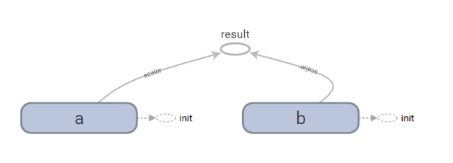
Running tensorboard using the command below, and opening the URL, we get a simple overview of the graph.
tensorboard --logdir=/tmp/summary
Naming and scopes
Sometimes when working with large models, the graph visualization can become complex. To help with this, we can define scopes using tf.name_scope to add another level of abstraction, in fact, we can define scopes within scopes as illustrated in the example below:
with tf.name_scope('primitives') as scope:
    a = tf.Variable(5, name='a')
    b = tf.Variable(10, name='b')

with tf.name_scope('fancy_pants_procedure') as scope:
    # this procedure has no significant interpretation
    # and was purely made to illustrate why you might want
    # to work at a higher level of abstraction
    c = tf.multiply(a,b)

    with tf.name_scope('very_mean_reduction') as scope:
        d = tf.reduce_mean([a,b,c])

    e = tf.add(c,d)

with tf.name_scope('not_so_fancy_procedure') as scope:
    # this procedure suffers from imposter syndrome
    d = tf.add(a,b)

with tf.Session() as sess:
    sess.run(tf.global_variables_initializer())

    print (sess.run(c))
    print (sess.run(e))

    fw = tf.summary.FileWriter("/tmp/summary", sess.graph)
Note that the scope names must be one word.
Opening this summary in tensorboard we get:
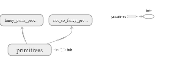
We can expand the scopes to see the individual operations that make up the scope.
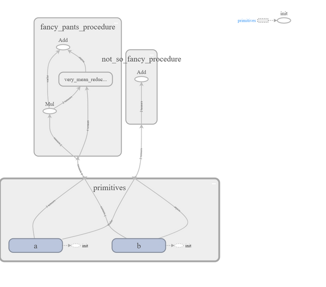
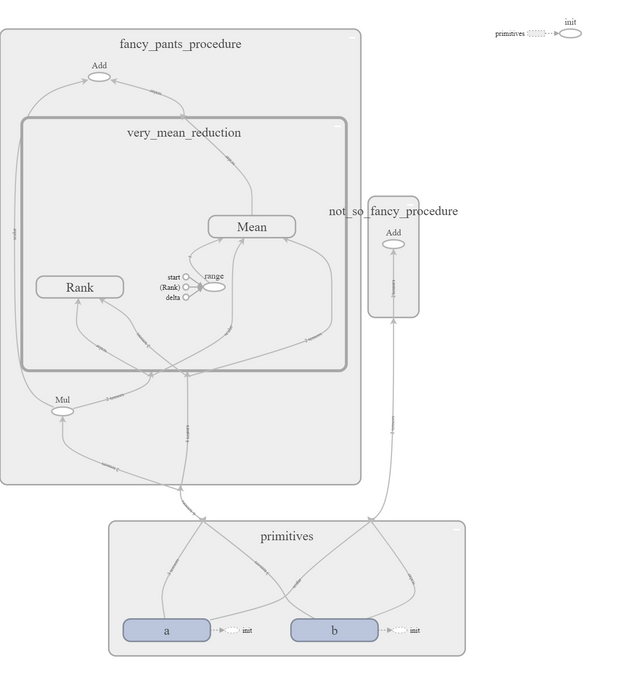
If we expand very_mean_reduction even further, we can see Rank, and Mean which are a part of the reduce_mean function. We can even expand those to see how those are implemented.
Visualizing changing data
While just visualizing the graph is pretty cool, when learning parameters, it'd be useful to be able to visualize how certain variables change over time.
The simplest way of visualizing changing data is by adding a scalar summary. Below is an example that implements this and logs the change of c.
import random

a = tf.Variable(5, name="a")
b = tf.Variable(10, name="b")

# set the intial value of c to be the product of a and b
# in order to write a summary of c, c must be a variable
init_value = tf.multiply(a,b, name="result")
c = tf.Variable(init_value, name="ChangingNumber")

# update the value of c by incrementing it by a placeholder number
number = tf.placeholder(tf.int32, shape=[], name="number")
c_update = tf.assign(c, tf.add(c,number))


# create a summary to track to progress of c
tf.summary.scalar("ChangingNumber", c)

# in case we want to track multiple summaries
# merge all summaries into a single operation
summary_op = tf.summary.merge_all()


with tf.Session() as sess:
    sess.run(tf.global_variables_initializer())

    # initialize our summary file writer
    fw = tf.summary.FileWriter("/tmp/summary", sess.graph)

    # do 'training' operation
    for step in range(1000):
        # set placeholder number somewhere between 0 and 100
        num = int(random.random()*100)
        sess.run(c_update, feed_dict={number:num})

        # compute summary
        summary = sess.run(summary_op)

        # add merged summaries to filewriter,
        # so they are saved to disk
        fw.add_summary(summary, step)
So what happens here?
If we start by looking at the actual logic, we see that the value of c, the changing variable, starts by being the product of a, and b (50).
We then run an update operation 1000 times which increments the value of c by a randomly selected amount between 0 and 100.
This way, if we were to plot the value of c over time, we'd expect to see it linearly increase over time.
With that out of the way, let's see how we create a summary of c.
Before the session, we start by telling Tensorflow that we do in fact want a summary of c.
tf.summary.scalar("ChangingNumber", c)
In this case, we use a scalar summary because, well, c is a scalar. However, Tensorflow supports an array of different summarizers including:
- histogram (which accepts a tensor array)
- text
- audio
- images
The last three are useful if you need to summarize rich data you may be using to feed a network.
Next, we add all the summaries to a summary op to simplify the computation.
summary_op = tf.summary.merge_all()
Strictly speaking, this is not necessary here as we only record the summary of one value, but in a more realistic example, you'd typically have multiple summaries which makes this very useful. You can also use tf.summary.merge to merge specific summaries like so:
summary = tf.summary.merge([summ1, summ2, summ3])
This can be powerful if coupled with scopes.
Next, we start the session where we do the actual summary writing. We have to tell Tensorflow what and when to write; it won't automatically write a summary entry every time a variable changes even though it'd be useful.
Therefore, every time we want a new entry in the summary, we have to run the summary operation. This allows for flexibility in how often, or with what precision, you want to log your progress. For example, you could choose to log progress only every thousand iterations to speed up computation, and free IO calls.
Here we just log the progress at every iteration with the following line of code:
summary = sess.run(summary_op)
We now have the summary tensorboard uses, but we haven't written it to disk yet. For this, we need to add the summary to the filewriter:
fw.add_summary(summary, step)
Here, the second argument step indicates the location index for the summary, or the x-value in a plot of it. This can be any number you want, and when training networks, you can often just use the iteration number. By manually specifying the index number, the summary writer allows for a lot of flexibility when creating the graphs as you can walk backwards, skip values, and even compute two, or more, values for the same index.
This is all we need. If we now open tensorboard, we see the resulting graph, and the plot that has been made from the summary.
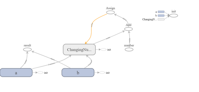
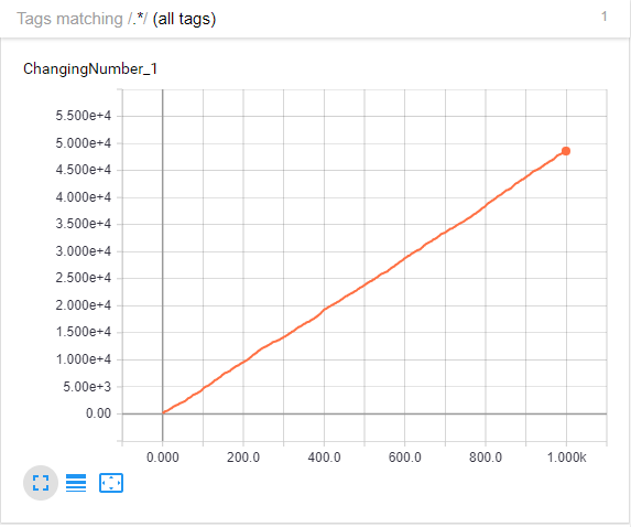
And as predicted, the trend of the summary plot is indeed linear with a positive slope.
Come back tomorrow for the last part where we will take everything we learned, and use it in a real example to create a small neural network.
Read part 5 here
I don't have the smallest idea what you are talking about, but seeing the work you put in this i am just amazed how the community did not support you more! If the effort is any indicator of the quality of your work, you soon will be discovered by flocks of people. And i am doing my share of supporting hardworking people. Kudos! :)
Thank you. It means a lot.
As for what I'm talking about, Tensorflow is a tool that helps you make machine learning (AI) models.
While the series does assume basic familiarity with common programming ideas, I've tried my best to make it approachable, so that people at any level can start from part 1, and at least understand the gist of what's happening.
Upvoted and RESTEEMED :]
Thanks.
Hello, Great stuff you have, Im following you now! :)
I am a live visual performer, using Arena Resolume for my shows, If you are interested follow me! :)
Thanks.
I really liked your glitch piece you made for the underground party.