Deep learning Note 2 — Part 2 Optimization
In my last post Deep Learning Note 2 — Part 1 Regularization I summarized some key points about regularization methods to improve deep neural networks. In this week I will summarize another two topics: Setup up your optimization problem and Optimization Algorithms. As a verification, my original post was published on my wordpress blog and I have stated in the original post that it is also published on Steemit. Pictures here are screenshots of the slides from the course.
Setup up your optimization problem
Assuming that we have defined our cost function, it’s time for us to jump right into optimize it, right? Well, not so fast. There are a few things to consider first.
Normalization
Before we feed the training data into the network, we need to normalize them (subtracting mean and normalizing variance as shown below) .
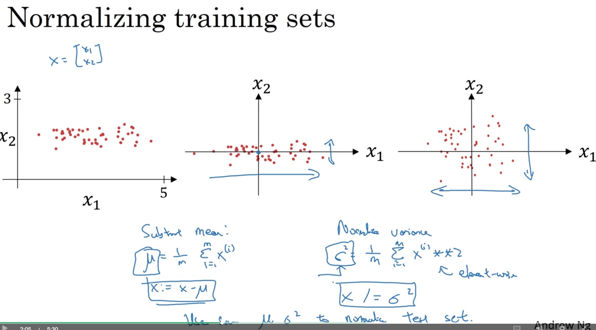
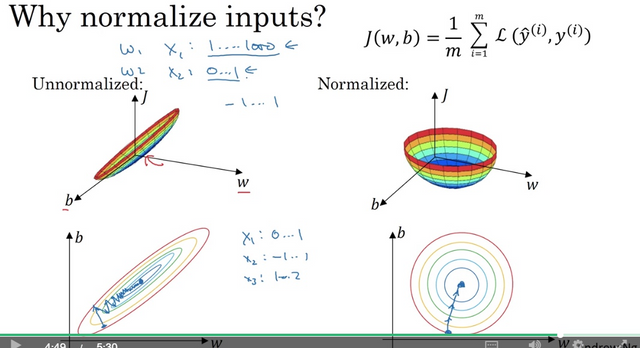
The advantage of normalization is that it makes it easier to optimize the cost function (in the way that we can supply a larger step size/learning rate to speed up the convergence).
One thing worth noting is that make sure to apply the normalization on the test and validation set using the mean and variance obtained on the training set. There is usually no harm of doing normalization on the input data so just do it.
Random weights initialization
One problem with deep neural network is the vanishing/exploding gradients that the derivative/slope can sometimes become very big or small which makes the training difficult.
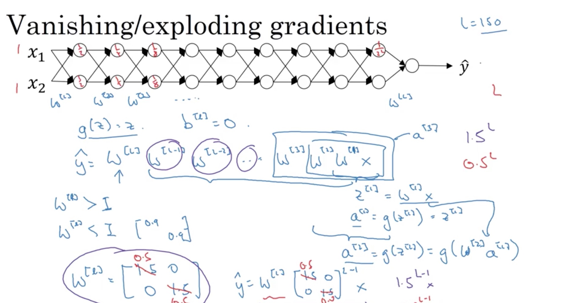
The screenshot above shows that if W is greater than 1, y will explode while if W is smaller than 1, y will vanish to a very small number. One way to (partially) solve this is to randomly initialize the weights, shown as follows:
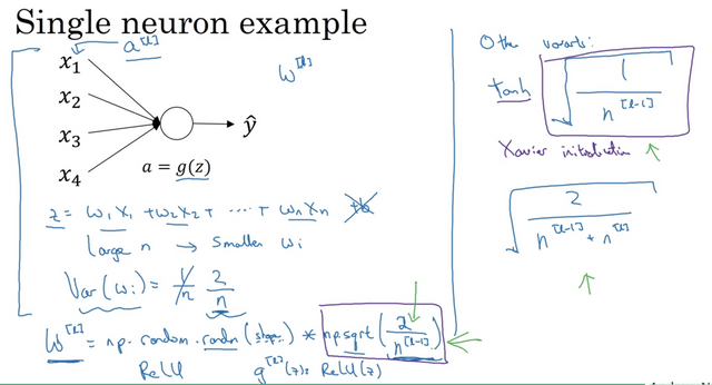
Using these scaling methods, W will not explode or vanish too quickly, which allows us to train relatively deep neural networks.
Gradient check
If we are implementing back-propagation ourselves, we need this check to make sure that our implementation is correct. To do that we need to do something called numerical approximation of gradients. For a simple function f(theta), the gradient at theta is
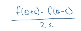
This version is more accurate than the [f(theta + epsilon) - f(theta)]/epsilon.
However, if we are just using deep learning frameworks, we don’t really have to do this. This is mainly for debugging the implementation of back-propagation if we are doing this on our own.
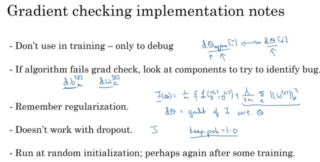
Things to watch out
- Gradient Checking is slow! Approximating the gradient is computationally costly. For this reason, we don't run gradient checking at every iteration during training. Just a few times to check if the gradient is correct. Then turn it off and use backprop for the actual learning process.
- Gradient Checking, at least as we've presented it, doesn't work with dropout. We would usually run the gradient check algorithm without dropout to make sure backprop is correct, then add dropout.
Optimization Algorithms
We’ve learned about one optimization algorithm--Gradient Descent (GD). There are other algorithms out there, mostly as an performance improvement of GD.
Batch VS. Mini-Batch VS. Stochastic Gradient Descent
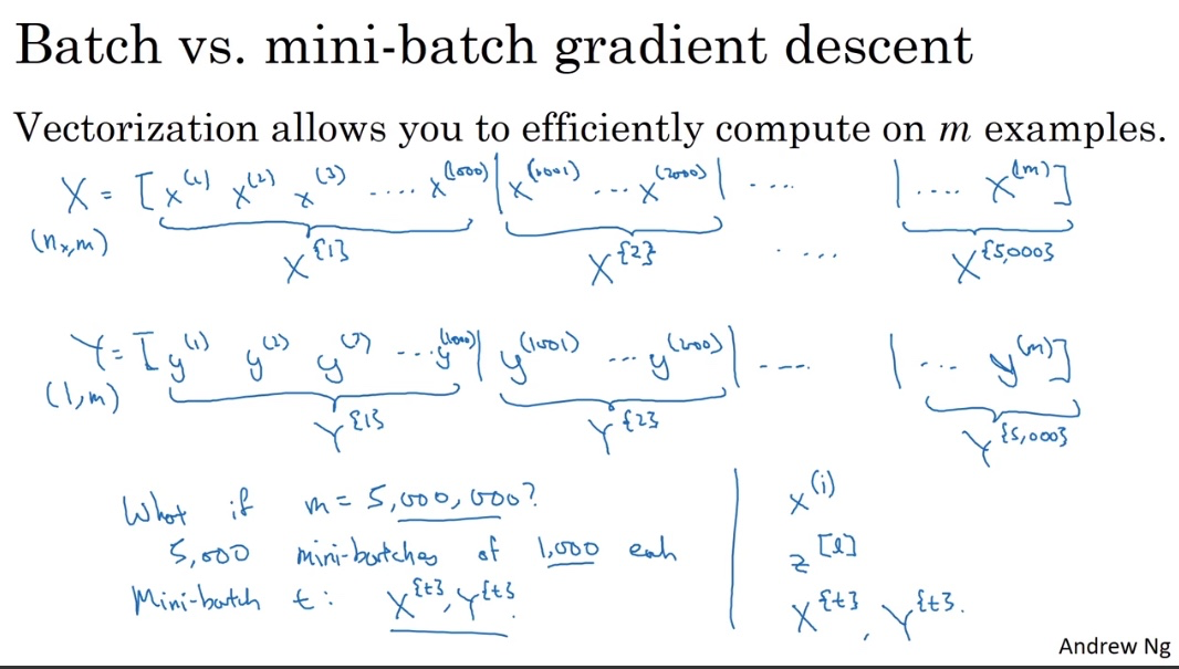
- Batch gradient descent uses the training data all at once in an epoch. Only one gradient descent in one epoch.
- Mini-batch, however, uses a subset of the training data at a time. Therefore, there are multiple batches of training and thus multiple steps of gradient descent in one epoch.
- SGD, to the extreme, uses 1 example at a time (batch_size = 1).
Why mini-batch GD?
Batch gradient descent is slow since it uses all data at once. SGD has high oscillation and loses the speed benefit of vectorization. Mini-batch is somewhere in between. It could show progress relatively fast and uses vectorization.
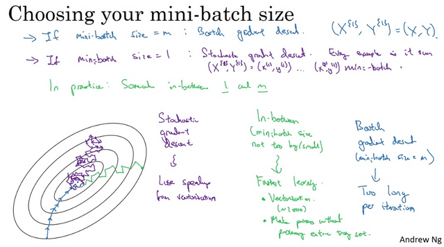
Why are there oscillations?
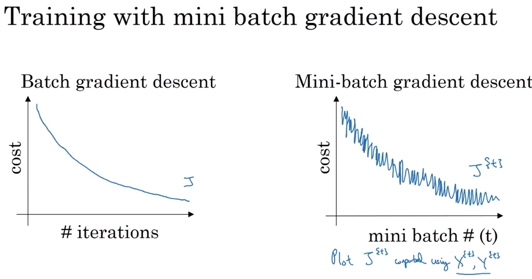
This is because that one batch may be easy to learn but the next one could be difficult. If we are using batch gradient descent and it diverges in even one iteration, that could mean we have a problem, for example, we set the step size too big.
Mini-Batch size
- If the training set size is small, don’t bother using mini-batch, just use the whole batch to train the network.
- Otherwise, shuffle the training data first and choose the batch size between 32 to 512 (power of 2) or whatever fits in the memory. If a particular mini-batch size has problem, check the memory cost.
Faster than Gradient Descent?
There are optimization algorithms faster than Gradient Descent: Momentum, RMSProp, and Adam. To understand them we need to use something called exponentially weighted average. It is the key components of those advanced optimization algorithm. The idea of these advanced algorithm is to compute a EWA (or some other forms of combinations) of the gradient and use that to update your weights instead. These algorithms have been proven effective in deep learning practices, especially the last two.
Exponentially weighted averages
I won’t go into much details but it is a way to approximate the average over the data in the last 1/(1-beta) days. In the screenshot below, the red line is the actual temperature while the green line is the moving average. The average line is smoother and it adapts slower when the temperature changes since it averages over a larger window of days. The larger beta is, the higher weight we gave to the previous days’ average and makes it less sensitive to changes in today’s data theta.
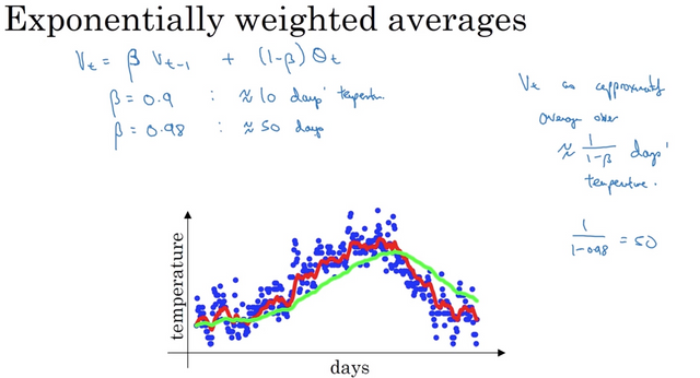
Note that this is just an approximation of the moving average (so it is less accurate) but it has the advantage of using less memory when computing since we don’t have to save the past X days’ of data. For efficiency purpose, this is widely used in machine learning.
Can it be more accurate?
There is a way to make it more accurate called **Bias correction **. If we use the original equation above, the average at the very beginning could be off (smaller) a lot to the real average. One way to do it is to divide the average by 1 - beta^t to compensate the offset at the beginning of the averaging line. When t is small, 1-beta^t is closer to o so it scales up the average. As t becomes larger, 1 - beta^t becomes closer to 1 and thus has less affect.
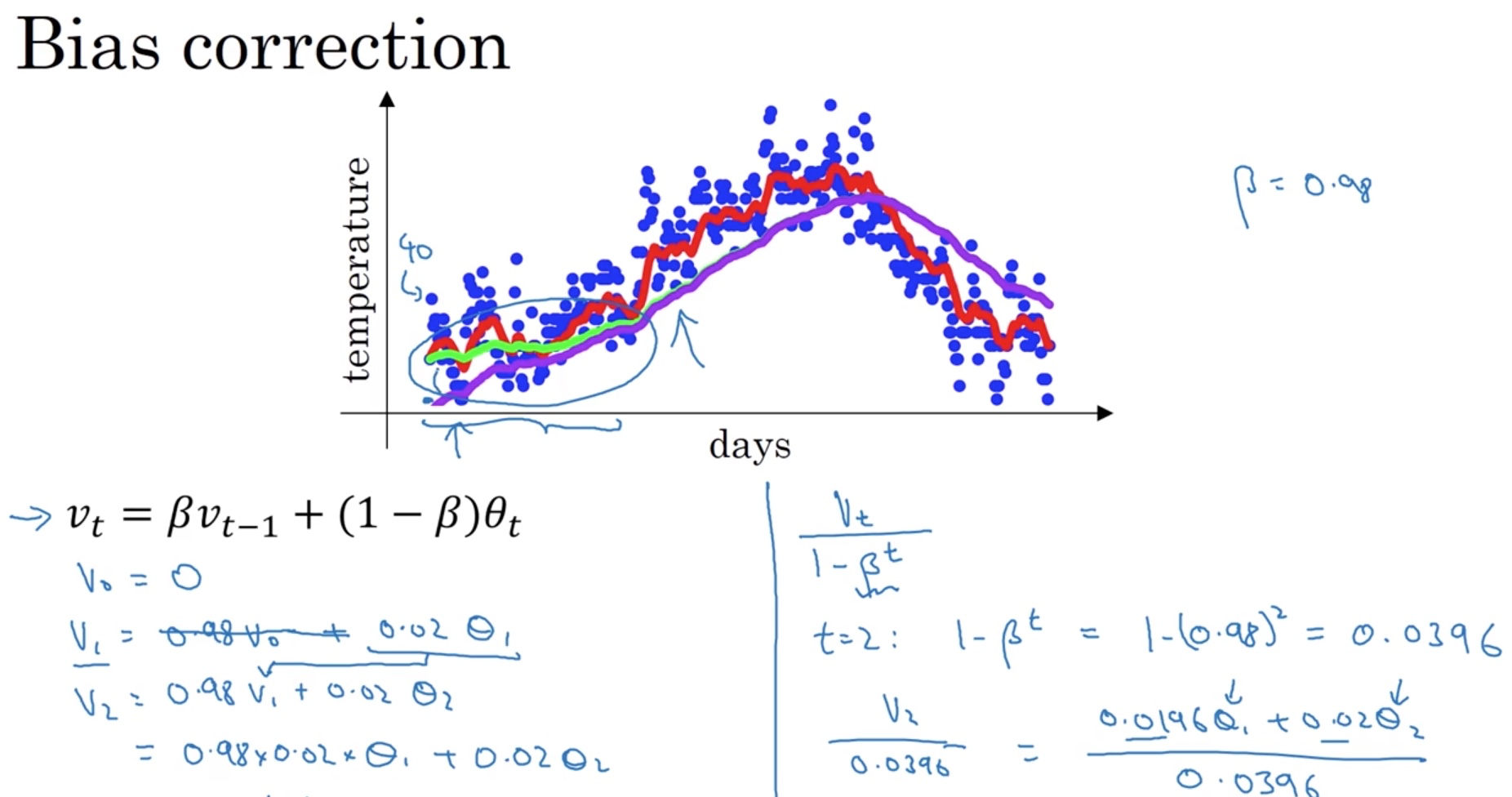
In practice, people often don’t bother to do bias correction. They would rather just wait for the initial period to pass. However, if you are concerned about the average at the beginning, bias correction is the way to go.
Gradient Descent with Momentum
The idea of momentum is to compute a EWA of the gradient and use that to update your weight instead. Let’s see an example to get an intuition of this algorithm.
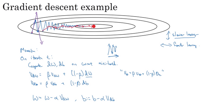
Gradient descent (the blue line) takes a lot of steps to get to the minimum. These up-and-down oscillation slows gradient descent down and prevent you to use a large learning rate (you may shoot too far on the wrong direction and end up diverging). On the horizontal direction, we want faster learning. Using momentum, we can achieve that goal. Since momentum is based on EWA, it can smooth out the oscillation on the vertical direction but keep the horizontal direction intact. In this way we move faster to the minimum and allows us to use a higher learning rate. Vdw and Vdb are both initialized to zeros.
Hyperparameters in Momentum
There are two parameters for Momentum. One is the learning rate alpha and the other is beta term we’ve seen in the EWA. A good default value for beta is 0.9 (about 10days average).
Summary
Momentum will almost always work better than gradient descent.
RMSprop (Root Mean Squre prop)
Similar to Momentum, RMSprop also updates the weight using some form of the EWA of the gradient, illustrated as follows:
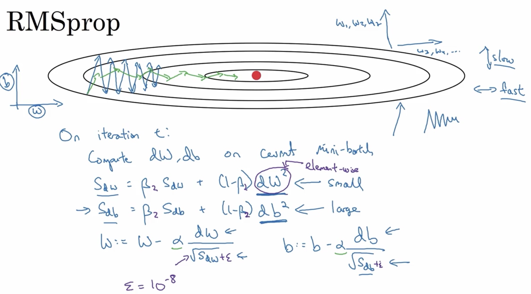
See the square of dW and the root square of SdW in purple? That’s where the name of Root Mean Square comes from. The intuition here is that for directions where the slope is large, Sd(W1, W2, W3...) will be large and cause smaller update (damping the oscillation) while for directions where the slope is small, Sd(W4, W5, W6...) will be small and cause larger update. This applies to both W and b here and note that W and b are both high dimensional. The example using W and b as the direction is a bit confusing though.
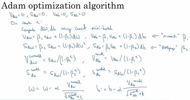
Adam
Adam combines the two algorithms above together as shown below. Not much to say here but it is proven to be very effective.
Summary
Based on the assignment of the course, we found that
Momentum usually helps, but given the small learning rate and the simplistic dataset, its impact is almost negligeable. Also, the huge oscillations you see in the cost come from the fact that some minibatches are more difficult thans others for the optimization algorithm.
Adam on the other hand, clearly outperforms mini-batch gradient descent and Momentum. If you run the model for more epochs on this simple dataset, all three methods will lead to very good results. However, you've seen that Adam converges a lot faster.
Some advantages of Adam include:
- Relatively low memory requirements (though higher than gradient descent and gradient descent with momentum)
- Usually works well even with little tuning of hyperparameters (except α )
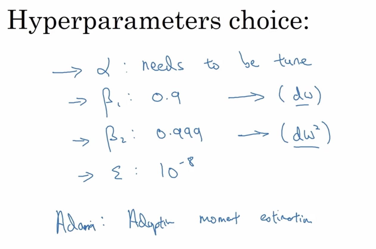
Hyper-parameter choices
These are the hyper-parameters for the Adam algorithm. In practice, people just use the default value of beta1, beta2 and epsilon. You still need to tune a set of alpha.
Learning Rate Decay
One way to speed up the learning process is to use learning rate decay. This sounds a bit counter-intuitive at first but here’s the explanation. The reason is that if we don’t reduce it, you may end up wandering around the minimum and never converge. The better way is to use large learning rate at first and then slowly reduce it. When you are around the minimum, you oscillate in a tighter region around the minimum rather than going off a lot.
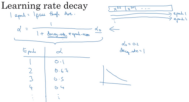
(Correction: the learning rate for the first epoch here should be the largest. Andrew might make a mistake here). There are some other ways of decaying the learning rate out there. Please refer to the note of CS231N. It has a very detailed explanation.
Local Optima?
People worry about their algorithm getting stuck at local minimum. However, the concept of this issue is changing in deep learning era.
Saddle Point
The issue is that if you are plotting a cost function with your weights in two dimensions, you do get a lot of local optima. But in training neural network, most points with zero gradients are not local optima. They are actually saddle points. See the difference between a bowl shape and a saddle shape on the left side of the slide in red.
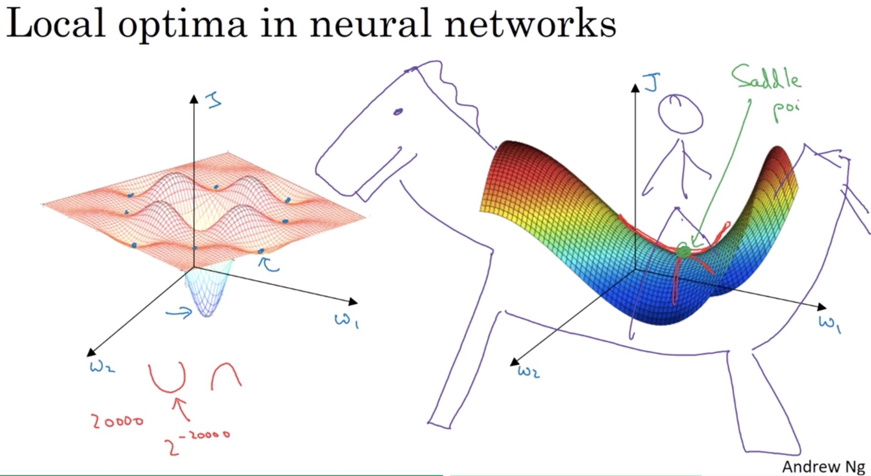
In high dimensional space, if you have 20000 dimensions, a real local optima requires all dimensions have a zero gradient of a bowl shape (rather than a saddle shape). The probability of that is 0.5^20000, which is very small. But seriously, it is a dinosaur, not a horse, right?
Congratulations @steelwings! You have completed some achievement on Steemit and have been rewarded with new badge(s) :
Click on any badge to view your own Board of Honor on SteemitBoard.
For more information about SteemitBoard, click here
If you no longer want to receive notifications, reply to this comment with the word
STOP