Looking at German Traffic Signs

A practical application of convolutional neural networks.
This article originally appeared on kasperfred.com
You know, I don't think we as a species do enough looking at German traffic signs.
I mean, sure, they are there when we drive through Germany, and we do (hopefully) see them, and sometimes we even register their meaning, and alter our behavior based on those meanings. But we don't do nearly enough looking at those bold, blue, red, and white, geometrical pictograms.
I think this is a shame, as by virtue of not looking, we do not appreciate their simplistic genius of interlingual communication.
That's why I decided to outsource all the looking to computers a while back when I was toying with an image classifier that would learn to classify traffic signs.
This will primarily be a commentary on what I did, and some ideas for what I could change, and do different in the future.
Since I used the Tensorflow library, I recommend reading my introduction to Tensorflow if you're not familiar with the library, or just need to catch up.
The dataset used was provided by the German Institute for Neuroinformatics (Institut für Neuroinformatik) under open access, and can be found here.
Before we begin, we start by importing the libraries needed, and check that all devices are recognized.
import os
import numpy as np
import matplotlib.pyplot as plt
import tensorflow as tf
from tensorflow.python.client import device_lib
from skimage import data as skimage_data
from skimage import transform
from skimage.color import rgb2gray

plt.style.use('ggplot') # make plots look better
def get_devices():
    local_device_protos = device_lib.list_local_devices()
    return [x.name for x in local_device_protos]

print (get_devices())
Next, we load the data. Since it came pre-split into a training- and a testingset, we will just use that as opposed to creating our own split.
Notice further that I didn't use the DataHandler described in the post mortem analysis. The reason for this is simply that I hadn't hit on the idea yet when doing this project.
def load_data(data_directory):
    directories = [d for d in os.listdir(data_directory)
                   if os.path.isdir(os.path.join(data_directory, d))]
    labels = []
    images = []
    for d in directories:
        label_directory = os.path.join(data_directory, d)
        file_names = [os.path.join(label_directory, f)
                      for f in os.listdir(label_directory)
                      if f.endswith(".ppm")]
        for f in file_names:
            images.append(skimage_data.imread(f))
            labels.append(int(d))
    return images, labels

ROOT_PATH = "./data"
train_data_directory = os.path.join(ROOT_PATH, "TrafficSigns/Training")
test_data_directory = os.path.join(ROOT_PATH, "TrafficSigns/Testing")

# load data
images_train, labels_train = load_data(train_data_directory)
images_test, labels_test = load_data(test_data_directory)
In order to use a static neural network, regardless of its architecture, the input dimensions must be the same for all examples. But as if often the case with images, the resolution of these can vary a lot between individual samples. So in order to use them, we have to standardize them before feeding the images to the network.
The simplest way of doing this is just to rescale all the images to a common resolution, and it turns out that this is not a bad approach either. Because the images are not of the same aspect ratio, we have to define a mode of interpolation, again, for simplicity, we just fill in black, an do not attempt to do any fancy interpolation which is evident by the use of the constant mode in the following code block.
While we could convert the images to grayscale as illustrated by the comment, we don't do this as the colors on the signs are specifically picked to convey information. Also, as we will find later, this is needed due to the poor distribution of the dataset.
# resize images
images_train = [transform.resize(image, (28,28), mode="constant") for image in images_train]
images_test = [transform.resize(image, (28,28), mode="constant") for image in images_test]

# convert to numpy arrays for efficiency
images_train = np.asarray(images_train)
images_test = np.asarray(images_test)

# convert images to greyscale
# images_train = rgb2gray(images_train)
# images_test = rgb2gray(images_test)
# when doing this, cmap must be set to grayscale when plotting the images
The 28 by 28 pixels were chosen because it's on the order of the resolution of most images, and because it's the resolution of the images in the common MNIST dataset.
To check that we have correctly imported the data, we can inspect the data dimensions to assure that we have correctly imported and rescaled the images.
print ("Trainingset:")
print ("img ndim: %d" % (images_train.ndim))
print ("number of images %d" % (len(images_train)))

print ("number of labels: %d" % (len(labels_train)))
print ("unique labels: %d" % (len(set(labels_train))))

print ("image shape", images_train[0].shape)

print ("\n")

print ("Testset:")
print ("img ndim: %d" % (images_test.ndim))
print ("number of images %d" % (len(images_test)))

print ("number of labels: %d" % (len(labels_test)))
print ("unique labels: %d" % (len(set(labels_test))))
Trainingset:
img ndim: 4
number of images 4575
number of labels: 4575
unique labels: 62
image shape (28, 28, 3)

Testset:
img ndim: 4
number of images 2520
number of labels: 2520
unique labels: 53
Here, it's seen that the number of unique labels are not same for the test and the training sets.
This poses a problem as the dataset is not large enough so that the test segment will test all the types of traffic signs. This means that the network could completely fail on the 9 types of signs that we're not testing, and it'd be difficult for us to find out, especially if it does well on the training data.
Furthermore, the measly ~4500 training examples are not a lot when considering that we will, as shown later, have several thousand features.
For more insight, we can look at the class distribution of the images.
# label distribution
plt.hist(labels_train, 62)

plt.show()
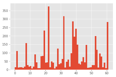
Here goes a similar story.
The large variance in the number of samples per label is also problematic as it will be difficult for a network to learn the representation for some of the classes for which there is not a lot of data.
I does, however, make sense that it'd be this way; that certain signs are a lot more prevalent than others as it reflects the real world distribution of the different signs.
This can be mitigated by just having a large amount of data, but as seen above, this is not the case, and as there's no simple way of getting more data, a lower accuracy is therefore to be expected, and it'll be difficult to fit a complex model, why a very deep neural network will likely not be ideal.
Continuing our exploration, now is probably a good time to do a visual inspection of the data:
traffic_signs = [300, 2250, 3650, 4000]

# Create subplots
for i in range(len(traffic_signs)):
    plt.subplot(2, 2, i+1)
    plt.axis("off")
    plt.imshow(images_train[traffic_signs[i]])

plt.show()
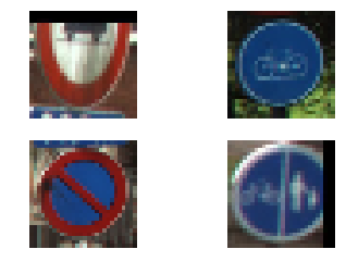
Here, we can visually see that the image transformation has worked, and that the images are padded with black bars as expected.
This can be extended to show an image for each class label with the code below.
unique_labels = set(labels_train)

plt.figure(figsize=(20,20))

i = 1

for label in unique_labels:
    image = images_train[labels_train.index(label)]

    plt.subplot(8, 8, i)
    plt.axis('off')
    plt.title("Label {0} ({1})".format(label, labels_train.count(label)))

    i += 1

    plt.imshow(image)

plt.show()
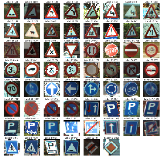
This does not only serve a useful lookup tables to figure out what sign-type the different labels represent, but also confirms our hypothesis that the differences in frequency of individual labels are correlated with the availability of these signs on the streets.
For example, while parking directions (label 40,41), and speed signs (label 32) are relatively common, signs signalling a specific height of a structure overhead (label 24,26,27) are relatively uncommon as expected.
Now that we have a pretty good understanding of the dataset, and its limitations, we can start creating our classifier model. Due to the quirks of the dataset, we will constrain the model to a single convolutional layer followed by two fully connected layers. For regularization, dropout is implemented.
If you aren't familiar with convolutional layers, you can read this introduction (coming soon).
Setting up the network graph can be done like so in Tensorflow:
def weight_variable(shape):
    initial = tf.truncated_normal(shape, stddev=0.1)
    return tf.Variable(initial)

def bias_variable(shape):
    initial = tf.constant(0.1, shape=shape)
    return tf.Variable(initial)

def conv2d(x, W):
    return tf.nn.conv2d(x, W, strides=[1, 1, 1, 1], padding='SAME')

def max_pool_2x2(x):
    return tf.nn.max_pool(x, ksize=[1, 2, 2, 1],
                        strides=[1, 2, 2, 1], padding='SAME')


x = tf.placeholder(dtype = tf.float32, shape = [None, 28, 28, 3])
y = tf.placeholder(dtype = tf.int32, shape = [None])
keep_prob = tf.placeholder(tf.float32)

# Input Layer
with tf.name_scope('input-layer') as scope:
    input_layer = tf.cast(x, tf.float32)

# conv layer 1
with tf.name_scope('conv1_layer') as scope:
    # reshapes dimensions to 28x28x64
    W_conv1 = weight_variable([5, 5, 3, 64])
    b_conv1 = bias_variable([64])
    h_conv1 = tf.nn.relu(conv2d(input_layer, W_conv1) + b_conv1)

    with tf.name_scope('pooling') as scope:
        # pooling 14x14x64
        h_pool1 = max_pool_2x2(h_conv1)

    with tf.name_scope('dropout') as scope:
        # dropout
        pool1_drop = tf.nn.dropout(h_pool1, keep_prob)


with tf.name_scope('fc1_layer') as scope:
    with tf.name_scope('flatten') as scope:
        # transition to fully connected layers
        pool1_flat = tf.reshape(pool1_drop, [-1, 14*14*64])

    # Fully connected 1
    W_fc1 = weight_variable([14*14*64,128])
    b_fc1 = bias_variable([128])
    h_fc1 = tf.nn.relu(tf.matmul(pool1_flat, W_fc1) + b_fc1)

    with tf.name_scope('dropout') as scope:
        # dropout
        fc1_drop = tf.nn.dropout(h_fc1, keep_prob)

with tf.name_scope('fc2_layer') as scope:
    # fully connected 2
    W_fc2 = weight_variable([128,64])
    b_fc2 = bias_variable([64])

with tf.name_scope('logits') as scope:
    # final logits
    logits = tf.matmul(fc1_drop, W_fc2) + b_fc2

loss = tf.reduce_mean(
    tf.nn.sparse_softmax_cross_entropy_with_logits(
        labels = y,
        logits = logits))

train_op = tf.train.AdamOptimizer(learning_rate=0.01).minimize(loss)

correct_pred = tf.equal(tf.argmax(logits,1), tf.argmax(y,1))
accuracy = tf.reduce_mean(tf.cast(correct_pred, tf.float32))
We can now train the network using the training operation. Notice that we don't use batch learning (stochastic gradient descent) due to the small size of the dataset.
tf.set_random_seed(42)

sess = tf.Session()

sess.run(tf.global_variables_initializer())
for i in range(201):
    _, loss_value = sess.run([train_op, loss], feed_dict={x: images_train, y: labels_train, keep_prob: 0.5})
    if i % 10 == 0:
        print("Loss: ", loss_value)
Loss:  11.8697
Loss:  3.3169
Loss:  2.24659
Loss:  1.56414
[...]
Loss:  0.187166
Loss:  0.168579
Loss:  0.166748
Loss:  0.154633
Again, the training error decreases in an inverse exponential manner as expected passing the acid test.
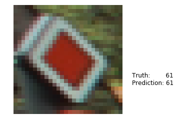
Individual samples can now be evaluated by evaluating the final layer's logits.
# predict a label of an image
sample_index = 3000

image = images_train[sample_index]
label = labels_train[sample_index]

pred = sess.run(logits, feed_dict={x:[image], keep_prob:1})
pred_label = list(pred[0]).index(max(pred[0]))

plt.axis('off')
plt.text(30,20, "Truth:        {0}\nPrediction: {1}".format(label, pred_label),
             fontsize=12)

plt.imshow(image)
plt.show()
We can extend this to look at a random sample to see what kind of predictions it gets right, and which it gets wrong.
import random

# Pick 10 random images
sample_indexes = random.sample(range(len(images_train)), 10)
sample_images = [images_train[i] for i in sample_indexes]
sample_labels = [labels_train[i] for i in sample_indexes]

pred = sess.run(logits, feed_dict={x: sample_images, keep_prob:1})
pred_labels = [list(pred[i]).index(max(pred[i])) for i in range(len(pred))]

# Display the predictions and the ground truth visually.
fig = plt.figure(figsize=(10, 10))
for i in range(len(sample_images)):
    truth = sample_labels[i]
    prediction = pred_labels[i]
    plt.subplot(5, 2,1+i)
    plt.axis('off')
    color='green' if truth == prediction else 'red'
    plt.text(30,20, "Truth:        {0}\nPrediction: {1}".format(truth, prediction),
             fontsize=12, color=color)
    plt.imshow(sample_images[i])

plt.show()
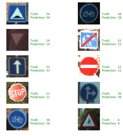
Of course, these samples are not representative of the final accuracy, we can find that, however, by:
# Run predictions against the full test set.
pred = sess.run(logits, feed_dict={x: images_test, keep_prob:1})
pred_labels = [list(pred[i]).index(max(pred[i])) for i in range(len(pred))]

match_count = sum([int(y == y_) for y, y_ in zip(labels_test, pred_labels)])
accuracy = match_count / len(labels_test)

print("Accuracy test: {:.3f}".format(accuracy))

# Run predictions against the full training set.
pred = sess.run(logits, feed_dict={x: images_train, keep_prob:1})
pred_labels = [list(pred[i]).index(max(pred[i])) for i in range(len(pred))]

match_count = sum([int(y == y_) for y, y_ in zip(labels_train, pred_labels)])
accuracy = match_count / len(labels_train)

print("Accuracy train: {:.3f}".format(accuracy))


# find examples of errors:
errors = []
index = 0
for pred,label in zip(pred_labels, labels_test):
    if pred != label:
        errors.append(index)
    index += 1

# Display the predictions and the ground truth visually.
fig = plt.figure(figsize=(10, 10))
for i in range(10):
    index = np.random.choice(errors)
    truth = labels_test[index]
    prediction = pred_labels[index]
    plt.subplot(5, 2,1+i)
    plt.axis('off')
    color='green' if truth == prediction else 'red'
    plt.text(30,20, "Truth:        {0}\nPrediction: {1}".format(truth, prediction),
             fontsize=12, color=color)
    plt.imshow(images_test[index])

plt.show()
Accuracy test: 0.950
Accuracy train: 0.998
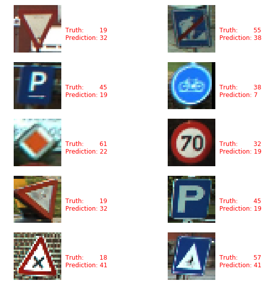
Here it's seen that the model works with a accuracy of 95% on the testset and 99.8% accuracy on the training set. The discrepancy between the testing and training error could be a sign of the network overfitting, and can be combated with more aggressive regularization, and, perhaps, by using fewer features, but this may also reduce the overall accuracy of the network.
One thing to notice from the types of errors plotted is that the network frequently predict label 19 over a range of different labels for example 32, and 45 shown here. Using the distribution plot above, we see that label 19 indeed is very common in the dataset, so this shows that the network fails to learn the representations of some of the less common classes, and overwrites them with the stronger representation of other signs. It's possible that permuting the data, and thus creating a larger synthetic dataset, will help alleviate the problem.
As a final touch, we will save the model, so that we can use it later.
saver = tf.train.Saver()
save_path = saver.save(sess, "/pretrained/model.ckpt")
print("Model saved in file: %s" % save_path)
Model saved in file: /pretrained/model.ckpt
Conclusion
While this is not the most sophisticated model, nor the dataset particularly friendly, the model actually does reasonably well with a 95% testing accuracy - which while not great isn't completely terrible either.
Moreover, this will probably mark the end of this project; one that I started a long time ago, but never had time to finish.
If you enjoy this informal kind of walkthrough, and you want me to do more of these, please let me know on Twitter.
Follow back n upvote me....
Please
Nice work men! you got my upvote (y)
Thanks
nice
Thanks
thanks for the knowledge is very useful for me
I'm glad that it helped.
Thank you for dropping by chat. I've added you to our content verification list.
https://steemcleaners.org/verified-user-lookup/entry/261383/
I apologize for the inconvenience.