R Programming - Text Analysis On Paul Van Dyk feat. Plumb - I Don't Deserve You Lyrics
Hi there. In this post, I do some text mining/analysis on the (trance/dance) music track I Don't Deserve You by Paul Van Dyk feat. Plumb. This project was done to fulfill my own curiousity.
There is also the version of this track by Plumb herself. The lyrics are similar except for one part and the Plumb track is more softer/mainstreamish compared to the Paul Van Dyk version.
This page contains some of the code and outputs. The full version can be found from my website here.

Good resources/references include the R Graphics Cookbook by Winston Chang and Tidy Text Mining With R Book By Julia Silge and David Robinson.
Paul van Dyk - I Don't Deserve You ft. Plumb (Official Video)
Plumb - Don't Deserve You
Sections
- Loading The Lyrics Into R
- Word Counts In Paul Van Dyk feat. Plumb - I Don't Deserve You
- Sentiment Analysis
Loading The Lyrics Into R
The lyrics for Paul Van Dyk feat. Plumb - I Don't Deserve You were taken from azlyrics.com. The lyrics were copied and pasted the lyrics into a .txt file.
For data manipulation, data visualization, word counts and text mining in R, I use the packages:
- dplyr
- tidyr
*ggplot2 - tidytext
(If you need to install a package, use install.packages("pkg_name"). in R)
# Text Mining On Paul Van Dyk feat. Plumb - I Don't Deserve You

# Lyrics From https://www.azlyrics.com/lyrics/paulvandyk/idontdeserveyou.html

# Load libraries into R:

library(dplyr)
library(ggplot2)
library(tidytext)
library(tidyr)
With the readLines() function in R, you can read in .txt files. I read in the lyrics .txt file into R and convert it into a data frame. The head() function in R allows for partial printing of an object.
# Read the lyrics into R:

dont_deserve_lyrics <- readLines("paulvanDyk_dont_deserveYou_lyrics.txt")

# Preview the lyrics:

dont_deserve_lyrics_df <- data_frame(Text = dont_deserve_lyrics) # tibble aka neater data frame

> head(dont_deserve_lyrics_df, n = 10)
# A tibble: 10 x 1
 Text
 <chr>
 1 You're the first face that I see
 2 And the last thing I think about
 3 You're the reason that I'm alive
 4 You're what I can't live without
 5 You're what I can't live without
 6
 7 And never give up
 8 When I'm falling apart
 9 Your arms are always open wide
10 And your quick to forgive
The key function that is needed for text analysis is the unnest_tokens() function. This function separates all the words in a text in a way that each row has its own word.
# Unnest tokens: each word in the lyrics in a row:

dont_deserve_words <- dont_deserve_lyrics_df %>%
unnest_tokens(output = word, input = Text)

# Preview with head() function:

> head(dont_deserve_words, n = 10)
# A tibble: 10 x 1
 word
 <chr>
 1 you're
 2 the
 3 first
 4 face
 5 that
 6 i
 7 see
 8 and
 9 the
10 last
Word Counts In Paul Van Dyk feat. Plumb - I Don't Deserve You
There are words in the English language that are not useful in terms of meaning. Words such as the, and, me, you, myself, and of makes sentences flow but carry little meaning/importance on their own.
An anti_join() from the dplyr package is used to remove stop words from the lyrics.
##### 1) Word Counts
# Remove English stop words such as the, and, me , you, myself, of, etc.
dont_deserve_words <- dont_deserve_words %>%
anti_join(stop_words)
# Word Counts:
dont_deserve_wordcounts <- dont_deserve_words %>% count(word, sort = TRUE)
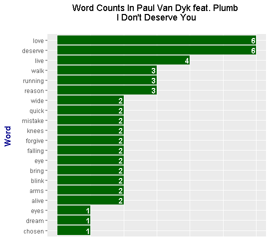
> head(dont_deserve_wordcounts, n = 15)
# A tibble: 15 x 2
word n
<chr> <int>
1 deserve 6
2 love 6
3 live 4
4 reason 3
5 running 3
6 walk 3
7 alive 2
8 arms 2
9 blink 2
10 bring 2
11 eye 2
12 falling 2
13 forgive 2
14 knees 2
15 mistake 2
From the head() output, the word deserve and the word love have a count of 6. To better display the results, it is preferable to use a bar graph from R's ggplot2 package.
# Plot of Word Counts (Top 20 Words):

dont_deserve_wordcounts[1:20, ] %>%
mutate(word = reorder(word, n)) %>%
ggplot(aes(word, n)) +
geom_col(fill = "darkgreen") +
coord_flip() +
labs(x = "Word \n", y = "\n Count ", title = "Word Counts In Paul Van Dyk feat. Plumb \n I Don't Deserve You \n") +
geom_text(aes(label = n), hjust = 1.2, colour = "white", fontface = "bold") +
theme(plot.title = element_text(hjust = 0.5),
axis.title.x = element_blank(),
axis.ticks.x = element_blank(),
axis.text.x = element_blank(),
axis.title.y = element_text(face="bold", colour="darkblue", size = 12))
Sentiment Analysis
In R's tidytext package, there are three main lexicons which analyze the sentiment/feelings of words. The three lexicons are nrc, AFINN and bing. The code and output below are from the three lexicons.
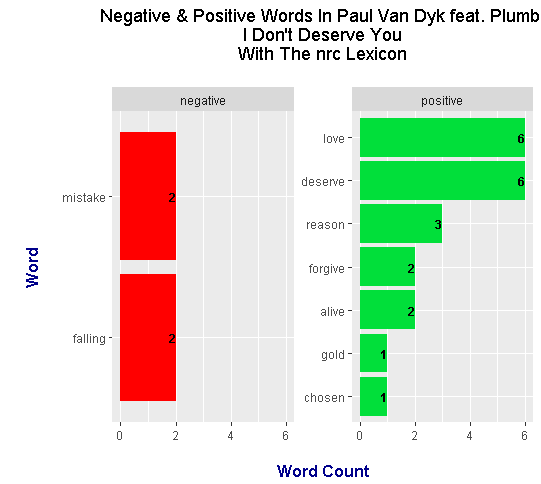
nrc Lexicon
##### 2) Sentiment Analysis:

# There are three main lexicons from the tidytext R package.
# These three are bing, AFINN and nrc.

### nrc lexicons:
# get_sentiments("nrc")

dont_deserve_words_nrc <- dont_deserve_wordcounts %>%
inner_join(get_sentiments("nrc"), by = "word") %>%
filter(sentiment %in% c("positive", "negative"))

> head(dont_deserve_words_nrc)
# A tibble: 6 x 3
 word n sentiment
 <chr> <int> <chr>
1 deserve 6 positive
2 love 6 positive
3 reason 3 positive
4 alive 2 positive
5 falling 2 negative
6 forgive 2 positive
# Sentiment Plot with nrc Lexicon

dont_deserve_words_nrc %>%
ggplot(aes(x = reorder(word, n), y = n, fill = sentiment)) +
geom_bar(stat = "identity", position = "identity") +
geom_text(aes(label = n), colour = "black", hjust = 1, fontface = "bold", size = 3.2) +
facet_wrap(~sentiment, scales = "free_y") +
labs(x = "\n Word \n", y = "\n Word Count ", title = "Negative & Positive Words In Paul Van Dyk feat. Plumb \n I Don't Deserve You \n With The nrc Lexicon \n") +
theme(plot.title = element_text(hjust = 0.5),
axis.title.x = element_text(face="bold", colour="darkblue", size = 12),
axis.title.y = element_text(face="bold", colour="darkblue", size = 12)) +
scale_fill_manual(values=c("#FF0000", "#01DF3A"), guide=FALSE) +
coord_flip()
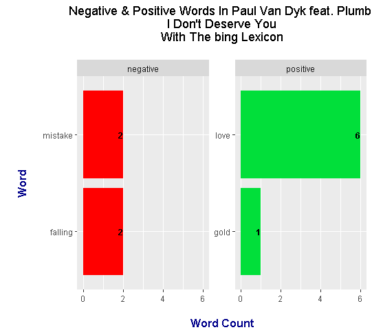
bing Lexicon
### bing lexicon:
# get_sentiments("bing")

dont_deserve_words_bing <- dont_deserve_wordcounts %>%
inner_join(get_sentiments("bing"), by = "word") %>%
ungroup()

> head(dont_deserve_words_bing)
# A tibble: 4 x 3
 word n sentiment
 <chr> <int> <chr>
1 love 6 positive
2 falling 2 negative
3 mistake 2 negative
4 gold 1 positive

# Sentiment Plot with bing Lexicon

dont_deserve_words_bing %>%
ggplot(aes(x = reorder(word, n), y = n, fill = sentiment)) +
geom_bar(stat = "identity", position = "identity") +
geom_text(aes(label = n), colour = "black", hjust = 1, fontface = "bold", size = 3.2) +
facet_wrap(~sentiment, scales = "free_y") +
labs(x = "\n Word \n", y = "\n Word Count ", title = "Negative & Positive Words In Paul Van Dyk feat. Plumb \n I Don't Deserve You \n With The bing Lexicon \n") +
theme(plot.title = element_text(hjust = 0.5),
axis.title.x = element_text(face="bold", colour="darkblue", size = 12),
axis.title.y = element_text(face="bold", colour="darkblue", size = 12)) +
scale_fill_manual(values=c("#FF0000", "#01DF3A"), guide=FALSE) +
coord_flip()
AFINN Lexicon
For the AFINN lexicon, I include a is_positive column with the mutate() function. This helps differentiate which words have positive scores and which ones have negative scores.
### AFINN lexicon:
# get_sentiments("afinn")

dont_deserve_words_afinn <- dont_deserve_wordcounts %>%
inner_join(get_sentiments("afinn"), by = "word") %>%
mutate(is_positive = score > 0)

> head(dont_deserve_words_afinn)
# A tibble: 6 x 4
 word n score is_positive
 <chr> <int> <int> <lgl>
1 love 6 3 TRUE
2 alive 2 1 TRUE
3 falling 2 -1 FALSE
4 forgive 2 1 TRUE
5 mistake 2 -2 FALSE
6 dream 1 1 TRUE
# Change labels
# (Source: https://stackoverflow.com/questions/3472980/ggplot-how-to-change-facet-labels)

labels <- c(
`FALSE` = "Negative Words",
`TRUE` = "Positive Words"
)

dont_deserve_words_afinn %>%
ggplot(aes(x = reorder(word, n), y = n, fill = is_positive)) +
geom_bar(stat = "identity", position = "identity") +
geom_text(aes(label = n), colour = "black", hjust = 1, fontface = "bold", size = 3.2) +
facet_wrap(~is_positive, scales = "free_y", labeller = as_labeller(labels)) +
labs(x = "\n Word \n", y = "\n Word Count ", title = "Negative & Positive Words \n In Fort Minor - Remember The Name \n With The AFINN Lexicon \n",
fill = c("Negative", "Positive")) +
theme(plot.title = element_text(hjust = 0.5),
axis.title.x = element_text(face="bold", colour="darkblue", size = 12),
axis.title.y = element_text(face="bold", colour="darkblue", size = 12)) +
scale_fill_manual(values=c("#FF0000", "#01DF3A"), guide=FALSE) +
coord_flip()
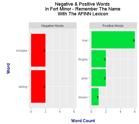
It turns out that the sentiment plots are not that interesting nor informative. The lyrics we have is a small sample size in terms of the amount of text. Regardless, this was a good exercise for practice and illustrative purposes.