Hey it's a me again! Today we get into a new math branch that I will cover with many many posts called Mathematical Analysis, where we will talk about functions, monotony, limits, derivatives, integrals, series, multi-variable functions and much more later on... Today's post actually has to do with almost the same stuff that we covered in Functions of Linear Algebra. We will get into some new stuff and I will also split this post in half so that we continue tomorrow...So, without further do let's get straight into it!

Functions:

    A function f from a non-zero set A to a non-zero set B is a rule f, that corresponds each element x of set A to only one specific element y of set B. We symbolize it as f: A -> B. We say that "f is a function from A to B".

    The element x is called the independent variable and y is the dependent variable or image of x and so we say that y = f(x).

    The set A of all x's is called the domain of definition and the set B of all images f(x) is called the domain of range of f.

The set of range of f: A -> B is:

f(A) = { foreach y in B there is a x in A so that: y = f(x)} = {f(x) : x in A}

    The sets A and B will mostly be real number sets (R) and so we will be talking about real functions with real values.

Example:

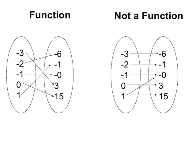
google image

The left one is a function, because each x corresponds to only one y. 

The right one is not a function, cause for x =1 we see that f(x) = 0 or 15.

ATTENTION: We can have multiple x's go to the same y (think about f(x) = c)

Some Function examples (will get into more later):

1. Constant functions of the type f(x) = c, where c is a real number. For c = 0 we have the zero-function.
2. Identity function of the type f(x) = x.
3. Polynomial functions of the type f(x) = an*x^n + an-1*x^n-1 + ... + a1*x + a0. The special case where n = 1 is called a Linear function: f(x) = a1*x + a0.
4. Rational functions of the type f(x) = P(x) / Q(X), where Q(X)!=0 and P, Q are polynomials.

Injective/Surjective/1-1:

    In Linear Algebra we called this kind of functions a mono, epi or isomorphism, but here we will get into a different naming!

Injective:

A function f: A -> R is injective when for every different value x in set A correspond different images f(x).

This means that for every x1, x2 in A we have that:

x1 != x2 <=> f(x1) != f(x2) (can be applied for equality too)

Surjective:

A function f: A -> B is surjective when the set of range f(A) matches with the set B.

So, we have that f(A) = B.

We could also say that every element of B is an image of at least one of the elements of set A.

This means that for every y in set B there is a x in set A so that f(x) = y.

1-1:

A function f: A -> B is 1-1 when it is injective and surjective at the same time.

We call these functions one-to-one.

Those functions have some special properties that we will get into in a bit.

All the linear functions are 1-1 tho.

Example:

Suppose the function f: Z -> N, where Z is the integer space and N is the natural number space.

For m in Z we have that:

f(m) = 0, m = 0

         = 2m, m > 0

         = -2m +1, m < 0

f is surjective cause:

• when x = 2n, there is a n in Z so that f(n) = 2n = x
• when x = 2n + 1, there is a -n in Z so that f(-n) = 2n + 1 = x

f is injective cause:

• when m1 != m2  <=> f(m1) != f(m2) always

    This means that f is 1-1 that could also be found by saying that f is a linear function after proofing that is is surjective.

Cartesian product:

For 2 elements a, b we define a ordered pair (a, b).

    Now, suppose A and B are non-empty sets. The set of all possible ordered pairs (a, b), where a is a element of A and b a element of B is called the cartesian product of A and B and is symbolized as:

AxB = {(a, b): a in A and b in B}

Example:

Suppose A = {a, b, c}, B = {1, 2}.

AxB = {(a, 1), (a, 2), (b, 1), (b, 2), (c, 1), (c, 2)}

and

BxA = {(1, a), (1, b), (1, c), (2, a), (2, b), (2, c)}

ATTENTION: AxB != BxA

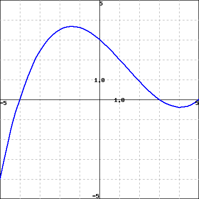
Function Graph:

Suppose A, B subsets of R and a function f : A -> B.

The set Gf = {(x, f(x): x in B} is a subset of AxB and is called the graph of function f.

    This graph can be represented in the 2-dimensional space and so with (x1, y1) and (x2, y2) being two random points in the 2d space we have that:
y2 - y1 / x2- x1 = a, where a is called the slope of function f.

    This number is equal to the tangent tan(ω), where ω is the angle of our line ε and the x axis in anticlockwise rotation.

Function Rules:

Suppose 2 function f: A -> R and g: B-> R then:

Equality

f: A -> R and g: B -> R are equal when:

• A = B
• f(x) = g(x) for any x in A (or B)

We symbolize equality as f = g.

Operations

1. h(x) = f(x) + g(x) <=> h = f + g is called the sum of the functions f and g
2. h(x) = f(x)*g(x) <=> h = f*g is called the product of the functions f and g
3. h(x) = c*f(x) <=> h = c*f, for c in R is called the product of f with number c.
4. h(x) = f(x)/g(x) <=> h = f/g, where g(x) != 0 is called the division of the functions f and g

Composition

Suppose f: A -> B and g: C -> D where A is subset of C.

The function h: A -> D for which:

h : A -> f(A) (through f) -> D (through g)

so that:

x -> f(x) = y (through f) -> z = g(y) = g(f(x)) = h(x) (through g)

is called the composition of f and g and is symbolized as gof.

Example:

Suppose the function f: R -> R, f(x) = x^2 + 1 and g: [0, +∞] -> R, g(x) = squareroot(x).

Because, x^2 >= 0 f(x) = x^2 + 1 >= 1 and so f(R) = [1, +∞]

So, the composition gof is:

g(x^2 + 1) = squareroot(x^2 + 1), where f(R)>=1 and so x is in R.

ATTENTION: gof != fog again as in the cartesian product.

Inverse function

Suppose f: A -> B a 1-1 function.

The function g: B -> A for which g(y) = x  for every y in B <=> f(x) = y

is called the inverse function of f and is symbolized as f^-1

Example:

Suppose f(x) = 2x +3.

The function is 1-1, because it is a linear function in the form f(x) = ax + b.

This means that y = f(x) = 2x + 3 => x = (y - 3) /2 

Switching the x, y's we have that:

f^-1(x) = y = (x - 3) / 2

Bounds:

Suppose a function f: A -> R.

1. f is upper bounded when there is a number M in R so that for every x in A  f(x) <= M. The minimum of those upper bounds is called the supremum of f (supf).
2. f is lower bounded when there is a number m in R so that for every x in A  f(x) >= m. The maximum of those lower bounds is called the infimum of f (inff).
3. f is bounded when lower and upper bounded.
4. f is absolute bounded when there is a positive num a in R so that for every x in A |f(x)|<= a (absolute value of f). The num a is called the absolute bound of f.
5. Any combination of absolute bounded functions is also absolute bounded.

Even-Odd Functions:

Suppose a function f: A -> R:

• f is a even function when for every x in A implies that -x is also in A and f(-x) = f(x). The graph is symmetrical to the y axis.
• f is a odd function when for every x in A implies that -x is also in A and f(-x) = -f(x). The graph is symmetrical to the center of the axes (0, 0).

And this is actually it for today and I hope you enjoyed it!

    Tomorrow we will continue with our Introduction of Functions getting into Monotony, Extremum and some more Categories of Functions.

Bye!