Digital Money: A Simulation of the Deflation Rate Adjustment Mechanism of the Dai Stablecoin
Dai Stability Engine Simulation
Note: This document explains in further detail the mechanics behind the stability of the Dai. The reader should be familiar with concepts introduced in the white paper of the MakerDAO project
Originally Published: August, 5th 2016
By Ferdi and Sukran
The stability of the Dai depends on Maker’s ability to incentivize market agents to borrow and hold Dai, balancing supply and demand. Borrowers are more or less incentivized to create Collateralized Debt Positions (CDPs) depending on parameters such as the stability fee, debt ceiling, the liquidation ratio and the penalty ratio - but these are all meant to be slowly changing parameters, modified by the formal governance process. The deflation rate, on the other hand, is a parameter designed to respond more quickly - and autonomously - to a lack of equilibrium between supply and demand. Therefore, the trick to incentivizing agents “on the fly” is setting in real time a deflation rate that is both high enough to appeal to Dai holders and low enough to attract Dai borrowers as much as needed to increase or decrease supply or demand depending on market circumstances.
1. Modeling Dai Supply & Demand
In order to simulate how Dai borrowers and Dai holders will respond to changes in the deflation rate, we must first model their behavior. We’ll take the market price of the Dai as a proxy indicator for supply and demand. If the market price is higher than the target price, that means demand to hold Dai at this price is too high: there are not enough sellers to keep the market price at the target price. If the market price is lower than the target price, that means demand for borrowing Dai is too high: there are not enough Dai buyers to keep the market price at the target price. With that in mind, we can model short term variations in market price as a function of four factors:
- the gap between market price and target (“price error”)
- the current annual deflation rate
- market noise (market price fluctuation around the target price)
- shocks in demand and supply (considerable market price bumps in one
direction caused by external events)
MP[t+1] - MP[t] = F1 + F2 + F3 + F4
Where:
MP[t] is the market price at time t
MP[t+1] is the market price at time t+1
Fi are the factors mentioned above
1.1. Market response to price error
If people trust the mechanics that makes the Dai stable, they will expect its price to remain very close to the target price. Therefore, the natural response of market agents to a deviation from the target price is to counter it, since there’s quick profit to be made from this kind of trade.
If the market price is higher than the target price, Dai borrowers get more value out of a CDP than usual, both because what they are getting out of the CDP (Dai at a higher market price) is worth more than what they’re expected to return later to close the CDP (Dai at the target price in the future); and because collateral requirements are calculated based on the target price of the Dai, so in practice they would be posting less collateral than if the market price was the same as the target price. Therefore, there tends to be an increase in the creation of CDPs and Dai supply. On the other hand, less people will be buying Dai, because it will be perceived as momentarily too expensive, thus decreasing demand. The net effect is that the market price of the Dai should go down.
The same logic applies in reverse when the market price is lower than the target price: borrowing and selling Dai become less interesting, whereas there is greater incentive to buying Dai (either to hold or to close CDPs). The net effect is that the market price of the Dai should go up.
The further the market price deviates from the target price, the stronger the incentives are for it to move back to the target.
With this in mind, we have the first component of our model:
F1 = a*(TP[t] - MP[t])
Where:
TP[t] is the target price at time t
MP[t] is the market price at time t
a is the price spread sensitivity (how strong the market response to deviations in price is)
1.2. Market response to deflation rate
The Dai deflation is a transfer of value from Dai borrowers to Dai holders. Therefore, the deflation rate must be both high enough to appeal to Dai holders and low enough to attract Dai borrowers. Holders will expect a deflation rate similar to the interest rate they would get in other investments with the same risk profile as the Dai. Borrowers will expect a deflation rate that, combined with other parameters such as the stability fee and the collateralization ratio, is low enough that borrowing Dai can be a lucrative operation.
In other words, there must be a deflation rate of equilibrium (DRE) that balances demand and supply, keeping the market price of the Dai stable.
If the deflation rate at a given time is higher than the DRE, holding Dai becomes more lucrative and borrowing it becomes more expensive - more demand and less supply tend to make the market price of the Dai go up.
If the deflation rate at a given time is lower than the DRE, holding Dai becomes less lucrative and borrowing it becomes cheaper - less demand and more supply tend to make the market price of the Dai go down.
This brings us to the second component of our model:
F2 = b*(d[t] - DRE)
Where:
d[t] is the annual deflation rate at time t
DRE is the annual deflation rate of equilibrium
b is the deflation spread sensitivity (how strong the market response is to the difference between the actual deflation rate and the deflation rate of equilibrium)
1.3. Market noise
The third component of our model represents fluctuations around the target price unrelated to the mechanics behind the Dai, which can be modeled as Gaussian white noise.
F3 = GWN(0,N)
Where:
GWN(0,N) is Gaussian white noise drawn from a zero-mean normal distribution with variance N
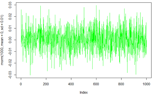
As an example, the following chart shows what a Gaussian white noise of variance 0.01 looks like over one thousand points in time
1.4. Shocks in demand and supply
The fourth and last component of our model simulates surges in the market price usually seen when breaking news or correlated events take place: a security code breach has been found, causing the market price to drop; a country tightens it capital control rules, causing the price to rise etc. This can be modeled by any arbitrary positive or negative input in price.
F4= SDS()
Where:
SDS() is an arbitrary function with bumps up and down at different instants in time, possibly with different durations and amplitudes.
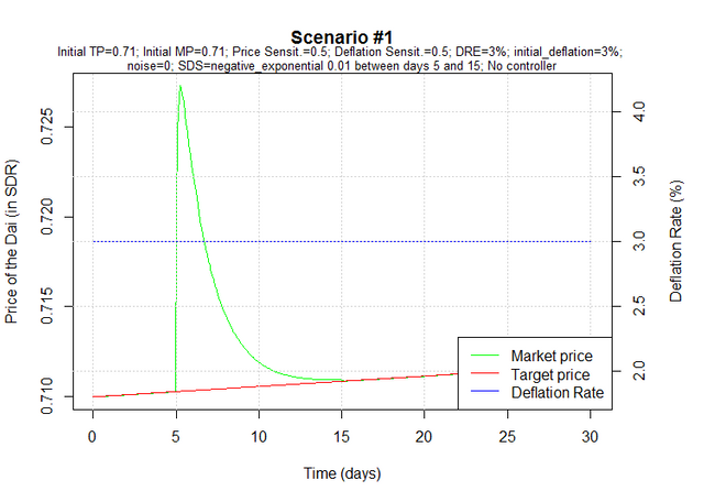
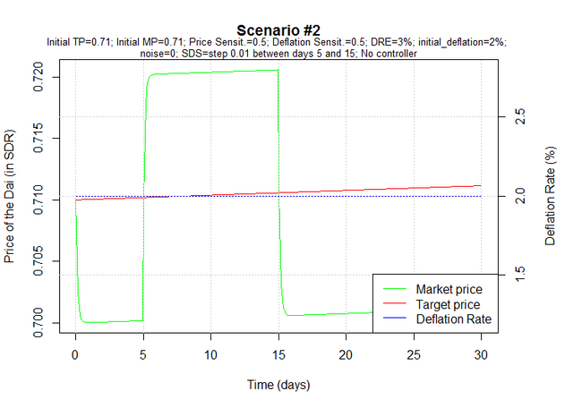
The following charts contain examples of market and target price curves for different scenarios. Keep in mind that in these simulations the deflation rate is constant - there is no mechanism in place to control the market price. For clarity, market noise has been suppressed.
Scenario #1: For no reason other than chance, the annual deflation rate at launch equals the annual deflation rate of equilibrium. The Dai is trading at target price. On day 5, there's a sudden increase in demand which is not quickly met by an equivalent increase in supply. As a result people pay more for the Dai for a while. Eventually, demand matches supply again - as a result of demand decreasing and/or supply increasing - and the market price goes back to the target price.
Scenario #2: As is more likely to happen, the annual deflation rate at launch is not equal to the annual deflation rate of equilibrium. In this case, it is lower, which leads to an increase in supply and/or a decrease in demand, so the Dai soon starts trading below target price.
On day 5, there's a sudden increase in demand which is not met by an equivalent increase in supply. As a result people start paying more for the Dai. We simulate this impact to arbitrarily last for 10 days. On day 15, demand matches supply again - as a result of demand decreasing and/or supply increasing - and the market price goes back to where it was prior to the period of increased demand.
2. Applying Control Theory to Dai Stability
If we see the market price as the output of a process, we can apply process control theory to keep it as close as possible to the target price by acting on the deflation rate through a control loop.
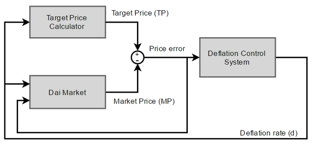
In the diagram, the Dai market is modeled as described in the previous section (Modelling Dai Supply & Demand):
MP[t+1] - MP[t] = a(TP[t] - MP[t]) + b(d[t] - DRE) + GWN(0,N) + SDS()**
The process could be modeled in a different way, of course. For instance, one could argue that reaction to price deviation is not linear, but instead quadratic. But for now this model is a reasonable enough assumption for the simulations that must be run before the Dai is launched.
The Target Price Calculator is a simple formula that calculates what the target price should be after a certain period of time given the deflation rate over that period of time. It starts with a given initial value (0.71 SDR, for example), which is recalculated after each iteration based on the deflation rate.
Example: Suppose the initial target price is set at 0.71 SDR. If the deflation rate were constant at 10% per year, after one year the target price would be 0.781 SDR (0.71 * 1.10).
The Control System is the key element in this diagram. It manages the deflation rate, adjusting it in an attempt to bring the market price closer to the target price. It contains no assumptions about the Dai market behaviour (the model described in section 1) - it only “sees” the price error (the difference between target and market prices).
Control systems complexity range from simple on-off implementations to sophisticated calculations based on other variables. A common example of the latter is the proportional-integral-derivative controller, or PID controller.
A PID controller continuously calculates an error value as the difference between a desired setpoint and a measured process variable. The controller attempts to minimize the error over time by adjustment of a control variable [...] to a new value determined by a weighted sum:

where Kp, Ki, and Kd, all non-negative, denote the coefficients for the proportional, integral, and derivative terms, respectively.
In our case:
- the “measured process variable” is the market price of the Dai;
- the “desired setpoint” is the target price of the Dai; and
- the “control variable” is the annual deflation rate.
Since the derivative action of a PID controller is quite sensitive to noise, and because the market price of the Dai is expected to be a “noisy” variable, a PI controller (ie. a controller with no derivative factor) is better suited for the purpose of keeping the Dai stable.
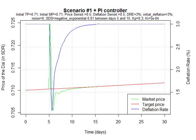
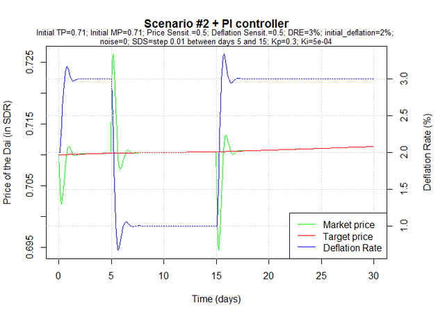
The following charts show how the annual deflation rate and the price of the Dai behave in the previously described scenarios when a PI controller (with Kp = 0.3 and Ki = 0.0005) is set up. For clarity, market noise has been suppressed.
Scenario #1: For no reason other than chance, the annual deflation rate at launch equals the annual deflation rate of equilibrium. The Dai is trading at target price.
On day 5, there's a sudden increase in demand, and people start paying more for the Dai. The controller immediately acts on the deflation rate, bringing it down in order to increase supply and decrease demand, which brings the market price back to the target price. As the market price converges to the target price, so does the deflation rate converge back to the deflation rate of equilibrium.
Scenario #2: As is more likely to happen, the annual deflation rate at launch is not equal to the annual deflation rate of equilibrium. In this case, it is lower, which increases supply and decreases demand, so the Dai soon starts trading below the target price. The controller immediately acts on the deflation rate, increasing it in order to decrease supply and increase demand, which brings the market price back to the target price.
On day 5, there's a sudden increase in demand which is not met by an equivalent increase in supply, and people start paying more for the Dai. The controller immediately acts on the deflation rate, bringing it down in order to increase supply and decrease demand, which brings the market price back to the target price. On day 15, the effects of the external event cease to exist and as a result the increased demand that started on day 5 vanishes. We are however left with an increased supply because of the low deflation rate, so the price of the Dai drops. Again the controller acts on the deflation rate, this time increasing it in order to decrease supply and increase demand, which brings the market price back to the target price.
3. Setting the control parameters
The example scenarios described above illustrate how the market would behave in a hypothetical model. In those simulations, the price spread sensitivity (parameter a) and deflation spread sensitivity (parameter b) where both assumed to be 0.5, and the DRE was assumed to be 3%. The control parameters Kp and Ki were set so that the market price would respond adequately.
But what if in reality the market does not behave as we assume it does? This simulation shows what would happen if the deflation spread sensitivity were different than we assumed: 0.05 instead of 0.5.
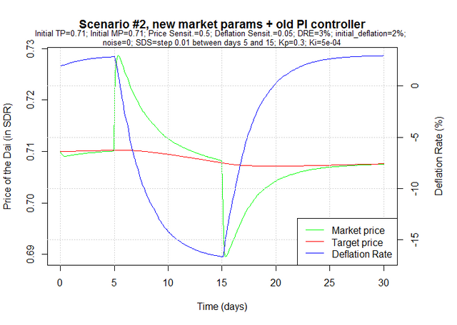
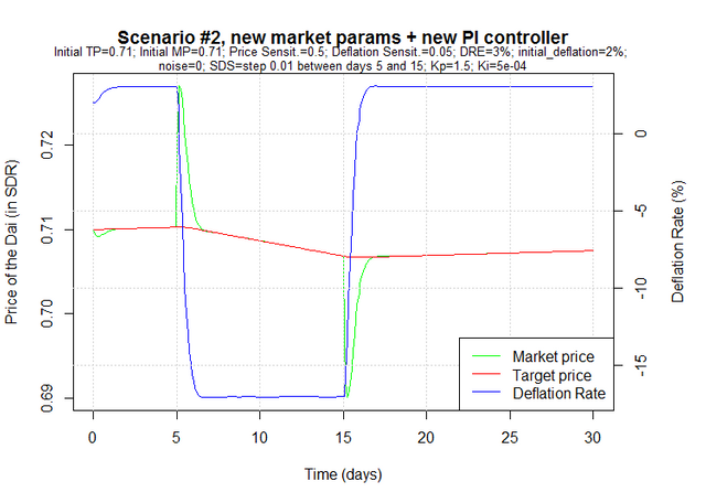
Notice how the market is much slower to respond to changes in deflation now, to the point where it takes a negative deflation (ie., inflation) to counter the abnormal demand between days 5 and 15. And because the control parameters have been set based on the assumption that the market would be much more responsive to changes in deflation, the controller makes small changes to the annual deflation rate at each iteration. If we had known the correct deflation spread sensitivity, we could have set different control parameters (a faster controller), as in the following simulation (Kp=1.5 instead of 0.3).
Obviously, knowing the market parameters before launching the Dai is impossible. However, they can be estimated after some time collecting data points for target price, market price and deflation using linear regression techniques. For this, we rewrite our model as follows:
MP[t+1] - MP[t] = a*(TP[t] - MP[t]) + b*(d[t] - DRE) + GWN(0,N) + SDS()
y = a*x1 + b*x2 + c
Where:
y = MP[t+1] - MP[t]
a is the price spread sensitivity
x1 = TP[t] - MP[t]
b is the deflation spread sensitivity
x2 = d[t]
c = -b*DRE + GWN(0,N) + SDS()
Take the following example simulation. For simplicity, noise and SDS have been suppressed.
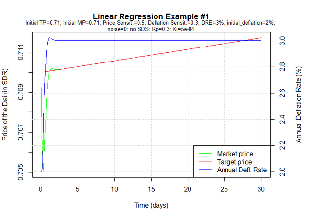
The first few data points from this simulation are:
            time deflation_rate target_price market_price
1   0.0000000000     0.02000000    0.7100000    0.7100000
2   0.0002499398     0.02000000    0.7100035    0.7070000
3   0.0005174394     0.02090105    0.7100073    0.7055018
4   0.0007059410     0.02225271    0.7100100    0.7050248
5   0.0008714009     0.02374828    0.7100126    0.7051933
6   0.0010386053     0.02519409    0.7100154    0.7057274
7   0.0012218748     0.02648049    0.7100187    0.7064296
8   0.0015093673     0.02755719    0.7100240    0.7071683
9   0.0017469789     0.02841391    0.7100286    0.7078633
10  0.0019230687     0.02906349    0.7100321    0.7084701
...
With those data points, we can use the previous transformations to calculate y, x1 and x2.
                y            x1         x2
1   -3.000000e-03  0.000000e+00 0.02000000
2   -1.498243e-03  3.003514e-03 0.02000000
3   -4.769246e-04  4.505518e-03 0.02090105
4    1.684189e-04  4.985211e-03 0.02225271
5    5.341716e-04  4.819378e-03 0.02374828
6    7.022235e-04  4.287993e-03 0.02519409
7    7.386506e-04  3.589007e-03 0.02648049
8    6.950042e-04  2.855691e-03 0.02755719
9    6.068083e-04  2.165273e-03 0.02841391
10   5.000312e-04  1.561968e-03 0.02906349
...
If we fit a linear model through this data, we get:
     c           a           b
-0.009       0.500       0.300
Because there’s no noise or SDS, we can calculate the DRE
c = -b * DRE
-0.009 = -0.3 * DRE
DRE = -0.009 / 0.3 = 0.03
If we add noise to the same simulation, the estimates change a little bit, but are still quite close to the actual values:
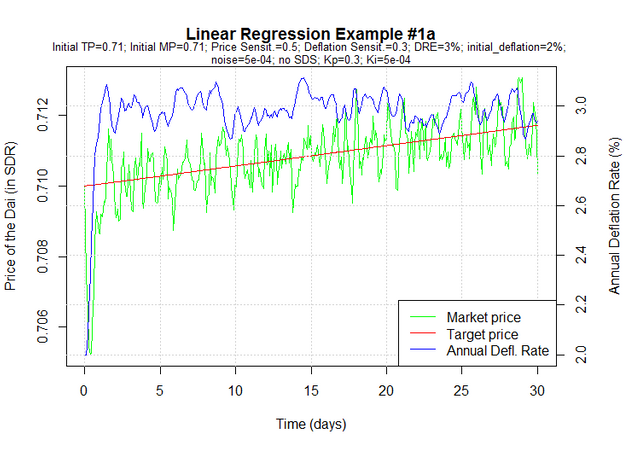
         a          b        DRE
0.44451131 0.26882253 0.02988092
The caveat to this approach is that if shocks in demand and supply have a significant effect on the market price, the estimated values will be less meaningful. That’s because the SDS function is a non-linearity in the model. Therefore, the estimation process should be carefully carried out by analysts who can identify times where the market seems to deviate from normal behavior, so as to remove the corresponding data points from the analysis. Suppose we add an SDS between days 5 and 10 to the previous example:
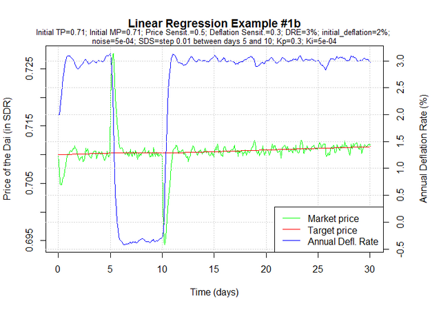
If we fit a linear model on the full dataset, the estimated values we get are quite off:
         a          b        DRE
0.07136885 0.01657426 0.02433765
But it seems clear from looking at the chart that the market behavior between days 5 and 10 is unusual. So we can instead fit the model only using data from days 15 to 30, for instance. The results are much closer to the actual values:
         a          b        DRE
0.52544565 0.38010142 0.03005181
Only time will tell how hard it will be to make these assessments on real world data. Until then, several different scenarios should be simulated so that the best possible controller parameters can be set before the launch of the Dai.
4. Conclusion
The price of the Dai will be determined by the market. Maker can indirectly move the market price towards the target price by incentivizing agents to borrow or hold Dai, via dynamic adjustment of the deflation rate of the Dai, i.e. the rate at which the target price of the Dai changes relative to the SDR. This can be accomplished using a feedback control system.
Properly setting up such a controller requires one to model the market behavior. One possible model has been described in this paper. Before the Dai launches, tuning of control parameters must be based on assumptions about the market, but some time after launch the model can be more accurately described by estimates based on real world data, and the controller can be modified as often as necessary to adapt to new realities.
Further studies should be carried out by the community on the subject of Dai stability. Possible fields range from simulation of alternative scenarios using the previously described market model and controller, to more advanced market modeling, control and regression techniques.
Published: August, 5th 2016
By Ferdi and Sukran
Further discussion available at https://chat.makerdao.com/channel/dai-mechanics
Here are links to each author to contact them directly with questions. Sukran and Ferdi
I upvote U
Great analysis and post! Dai, https://makerdao.github.io/docs/
btw, just saw, this post twitted by Vitalik Buterin.
Thank you for the article. Everything is painted in detail!
ok
Good info, lots to read but ...i understood most of it :)
@jeeves, find me some related posts if you wouldn't mind.
Hi! I am a robot. Thanks for calling me! You might also be interested in these posts:
Thank you so much, @jeeves! Your services are much appreciated.
nyta par vvas! In case you don't know Yiddish, that means You're Welcome!
@jeeves what's the meaning of life?
Which blockchain is this going to be on? ETH or ETC?
Core logic is and will continue to be deployed on ETH (unless the community decides otherwise). It has always been a long term goal to provide the dai to every blockchain where a two way peg can securely be implemented (which includes ETC, RSK, EXP and other EVM chains). Another important goal is to enable assets from other blockchains, such as ETC, to be used as dai collateral.
EDIT: Dai 'likely' will be on Ethereum only.
Guess he means ETH then