How I created a WINNING fantasy football prediction algorithm using Bayesian Modeling - The first stop on my journey [~7 min. read, original content and analysis]
Part 1: How to Determine Consistency
I was introduced to daily fantasy sports (DFS) like just about everyone- rapid fire commercials bombarding me on sportsball television. Fantasy sports was not a new concept to me, I’ve been a player since 1998. I cannot even begin to describe the countless hours I spent meticulously preparing draft guides for rotisserie baseball, basketball, and my personal favorite, football.

I had fun playing, at first. One of my favorite ways to think about DFS is it’s like renting your favorite team for a day. Let’s be honest, football games can be just brutal to watch if you aren’t cheering for your favorite team. Want proof? Try watching some Canadian football. I guarantee you don’t last for more than 5 minutes if you live south of Saskatchewan. So, DFS gave me another way to go through Sunday’s with more fun.
Bayesian statistics are my bae
I guess it was around the middle of last football season when things finally started to click in my head. First, the scandal where inside information helped a FanDuel employee win a DraftKings tournament. I should have known prior but I can have a thick head — knowing the percent a player is picked DOES matter. Why? So you can select someone that is not them; it sets you apart from the field.
Sometime thereafter, I read a really cool website outlining the gamma distribution and its nice fit with fantasy football data. This is where things REALLY started to click for me. So armed with a database of player data since 2003 and my trusty R, I went to work.
It turns out when you take a Bayesian approach, meaning you use data you have derived from previous weeks to help make predictions for future weeks, you can mathematically derive nice curves that help fit your data and make predictions. It’s like going to a gym: The more one trains themselves, the more one can make reasonable predictions of relative future fitness.
Bayesian analysis means making assumptions based on prior outcomes. Once you have a few prior outcomes they fit very nice curves to such outcomes to make predictions on future outcomes. Once a future outcome has taken place it is now a past outcome, and the nice fitting curve gets adjusted to reflect the new information.
Trust me, there is a lot of math behind this that would just make your head spin. Perhaps I will punt that to a future blog post.
However; for now, I would like to make a case for the Gamma Distribution as a really nice fit for predicting consistency in players’ fantasy football performances. Every graph and analysis below is my own.
Aaron Rodgers
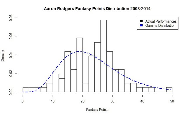
Consider the case of Aaron Rodgers. Below is a chart of every Aaron Rodgers fantasy performance over a seven year time period. The bars represent the percentage of times he scores a certain amount of points. The dotted blue line is his Gamma Distribution that models his data.
So, you can see from the tallest bar, he scores 25 points in about eight percent of his games. Pretty impressive!
What is more impressive, however, is his Gamma curve analysis. The chart below highlights Aaron Rodger’s quantiles. Red is the 0–25th quantile range, Yellow the 25–50th quantile, Green the 50–75th quantile. Think of these in terms of expectations. Yellow is an average performance, red below average, green above average.
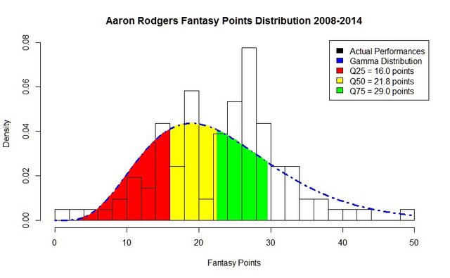
This set of data is now considered our training set. We can use this to make a prediction of the actual next performance.
Want to guess how many fantasy points Aaron Rodgers scored Week 1 last year?
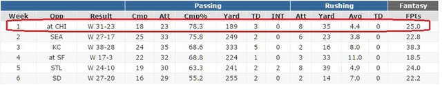
He scored 25 points. This puts him pretty close to his training set data average and firmly in the green zone. He had an above average performance for himself, but not quite his best ever. In a Bayesian model, we take this information, add it to our training set, and use it to make a prediction on Week 2.
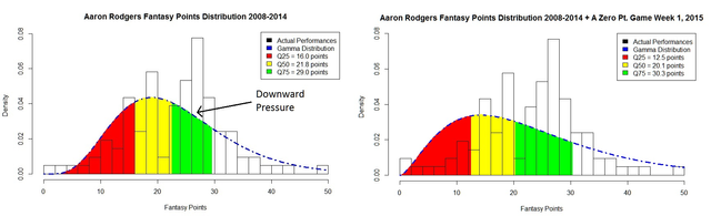
Extreme Examples
Just for funsies, what if Aaron Rodgers scored zero points in Week 1 against the Bears? Which - let’s face it - would have been extremely unlikely considering he was up against the Bears. If we apply this to our training data, we apply downward pressure on the gamma distribution, thus altering his quantiles for his next week. Essentially, we “smush” down the curve to the left to adjust for the putrid performance:
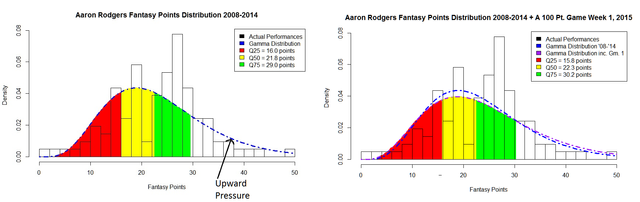
What about an awesome game? Say Aaron Rodgers scores 100 points. You guessed it, we apply upward pressure on the curve to the right as follows:
What does this all mean?
It means this is the start of what is an awesome predictive model. It does have its limitations though in terms of accuracy week to week, which is something I would like to outline in future posts to come. Here's a sneak preview though of how good it gets:
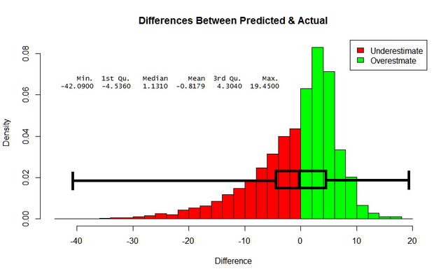
See that average below 1? Means I'm getting more or less within 1 point on average of an actual performance week to week!
What do you think Steem? The above represents my first blog post in what I hope to be a multi-part series of posts on my journey through fantasy predicive algorithms I am looking forward to launching this year. Any feedback you have for me would be appreciated!
#writing #blog #fantasyfootball #math #bayesian #analysis #steemit #sports #nfl #statistics #steem
Always been a fan of bayesian statistics, though I used the frequentist view for convenience. I used to place positive EV bets on illiquid betting exchanges, my stats are a bit rusty though!
It looks interesting but I don't fully get what you are trying to predict. Could you explain me a little bit better what you want to predict ? I might be able to help you with some future ideas.
I want to use the set of prior information on fantasy performances to build a model to predict future performances. I can use those predictions to influence my daily fantasy lineup I enter on a daily fantasy website, hopefully outperforming the statistically challenged.
This approach I outline is a good start, but does have its limitations that you can improve upon when considering other factors. I have found, it is pretty darn good at forecasting the consistency of a player.
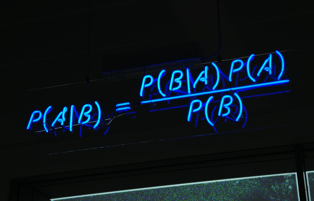
So you are trying to model the following, right ?
P(A|B) = P(Fantasy points prediction next week | Fantasy points this week)
Correct. Modeling the training set with the gamma distribution and selecting a likely to happen quantile value as their "B" value. Generating "A" values with many other high leverage football factors (red zone %, snaps, etc.).
Ok , cool. The gamma distribution looks quite weird though. It isn't really fitting the density in the region with highest probabilities. So the region that occurs most frequently is completely underestimated by the gamme distribution. Any idea why this is ? Is this an artefact of having chosen a small sampling size ?
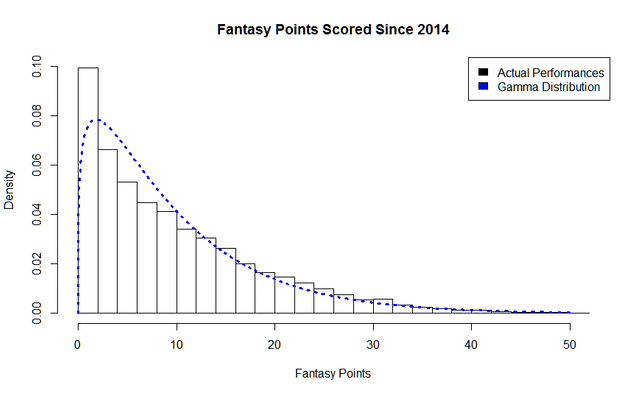
Tried to reply to the last comment of yours below but couldn't. Yes, this is completely due to sample size. This was trained from 103 performances, which is a lot, but not as robust as, say, all performances since 2014 for all players (the lead picture from the story).
Ok. Things are getting clearer to me :-).
You know what might improve the model ? At this moment you are modeling the following:
P(Performance this week | Performance last week).
Did you already try to model the following ?
P(Performance this week| Performance last week, Performance 2 weeks ago, Performance 3 weeks ago, ...)
You could take more past performances into account. This is what control engineers do when they model a system. The more you go backwards, the higher the order of the system. In order to determine amount of weeks you have to go back, you need gradually increase the order of your model and test its performance on a test set that you didn't use for training. Normally, in the beginning increasing the order could improve your model. But at some point increasing the order, will make your model worse. Than is when you know you don't have to increase the order anymore.
What do you think about this idea ?