R programming for quantitative investment: part 1 - fetch market data from web [originally posted in #crptocurrency]
[Originally posted in #cryptocurrency; I'm now posting in #programming after being recommended]
Fetch crypto price chart data from web and analyze data with Excel, R and other programs
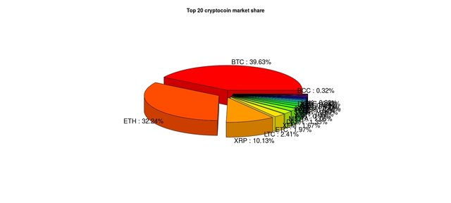
In this post we'll learn to use R to "read" web data and, as an illustrative application, use the data to plot a simple pie chart. I have been writing about a secure trading platform first before writing about trading strategies themselves. Instead of writing an intro-to-R type of post, I actually wanted to start with an application so the usefulness for the language is better realized. R users might find the post trivial; we'll soon write about advanced forecasting strategies with R's Finance and Time Series Analysis packages and other advanced techniques. Most important, we need data to conduct any kind of analysis. Here we'll learn to collect web data. For beginners, well, I guess to be able to plot - just with a few key strokes - with, say, R pietop20.R command, in couple of seconds - the below pie chart of percent of market share of top 20 (or any number) currencies should be enough motivation to learn R (or web scraping with other languages). I'm new to R - I will write as I learn. Suggestions and recommendations are much appreciated.
It looks cool, right? We can plot not only cool but also useful plots. If you don't understand the code now, just get along and get the concept. We'll talk about specific commands in other posts. I will leave links to resources I found helpful. If you don't want to install R, use SageMath online R console. So let's do it...
We'll "read" CryptoCurrency Market Capitalizations (CMC) price chart from their website and then analyze the data: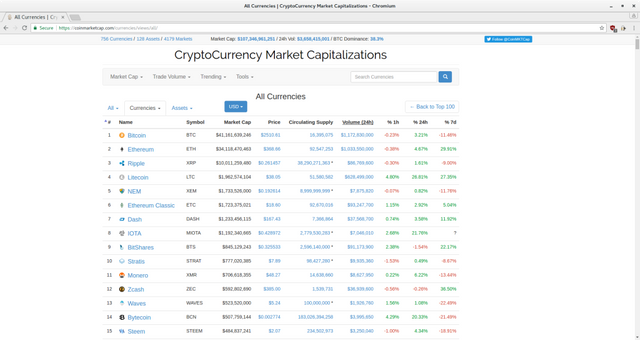
First load R packages, rvest, plotrix and dplyr. url_cmc is CMC price chart URL. In the code, texts entered after # are comments and ignored by R.
R> url_cmc <- "https://coinmarketcap.com/currencies/views/all/"
R> library(rvest) # for data fetching
R> library(plotrix) # for 3Dplot
R> library(dplyr)
Now do the actual reading:
R> url_cmc %>%
   read_html() %>%
   html_nodes(css = "table") %>%
   html_table() %>%
   as.data.frame() -> "tbl_cmc" # save table to variable <tbl_cmc>
The above code snippet "reads" crypto price chart and stores it to the variable named tbl_cmc.
Let's see what our program fetched by issuing head(tbl_cmc) command:
R> head(tbl_cmc)
  X.             Name Symbol      Market.Cap     Price                                                                    Circulating.Supply   Volume..24h.  X..1h X..24h   X..7d
1  1          Bitcoin    BTC $42,533,685,929  $2593.64                                                                            16,399,225 $1,122,030,000 -0.10%  0.76% -10.30%
2  2         Ethereum    ETH $34,637,433,018   $374.00                                                                            92,613,953   $688,324,000 -0.24% -1.57%  -1.84%
3  3           Ripple    XRP $10,845,834,234 $0.283253 38,290,271,363\n                    \n                    \n                        *   $253,494,000  0.12%  4.85%   6.05%
4  4         Litecoin    LTC  $2,584,999,454    $50.08                                                                            51,617,607   $991,078,000 -0.30% 14.08%  59.22%
5  5 Ethereum Classic    ETC  $2,112,575,943    $22.78                                                                            92,744,703   $249,724,000 -0.95%  1.48%   3.51%
6  6              NEM    XEM  $1,806,894,000 $0.200766  8,999,999,999\n                    \n                    \n                        *     $8,277,050  0.27%  2.42%  -9.58%
It did fetch the table, but the table contains a few unwanted characters such as new line, \n, spaces, %. In order to conduct analysis, we need to get rid off these characters. Computers don't seem to go well with texts; they understand numbers better. I would like to remove the first column(coins' ranking from CMC - we'll create rankings based on our custom criteria), make the column names small, lowercase and meaningful. Having a look at the website should make this post's naming. Let's do...
R> tbl_cmc[] <- lapply(tbl_cmc, gsub, pattern = "\\\n|\\s|[%*$,?]", replacement = "")
R> tbl_cmc$X. <- NULL
R> names(tbl_cmc) <- c("name", "symb", "mcap", "price", "supply", "vol", "ch1h", "ch24h", "ch7d")
See how our table looks with head(tbl_cmc):
R> head(tbl_cmc)
             name symb        mcap    price      supply        vol  ch1h ch24h   ch7d
1         Bitcoin  BTC 42533685929  2593.64    16399225 1122030000 -0.10  0.76 -10.30
2        Ethereum  ETH 34637433018   374.00    92613953  688324000 -0.24 -1.57  -1.84
3          Ripple  XRP 10845834234 0.283253 38290271363  253494000  0.12  4.85   6.05
4        Litecoin  LTC  2584999454    50.08    51617607  991078000 -0.30 14.08  59.22
5 EthereumClassic  ETC  2112575943    22.78    92744703  249724000 -0.95  1.48   3.51
6             NEM  XEM  1806894000 0.200766  8999999999    8277050  0.27  2.42  -9.58
Nice! We now have pretty nice looking table. Suppose, we're interested in top 100 crytocoins of total market capitalization. In order to select top 100, we can sort (descending) market capitalization, tbl_cmc$mcap. Oh, wait, can we run mathematical operations on market capitalization variable, mcap? Let's see:
R> typeof(tbl_cmc$mcap)
[1] "character"
We can't do maths on texts. Let's convert the character type to numeric:
R> num_tbl_cmc <- lapply(tbl_cmc[-c(1:2)], as.numeric) %>%
  as.data.frame()
R> tbl_clean <- cbind(tbl_cmc$name, tbl_cmc$symb, num_tbl_cmc)
R> names(tbl_clean) <- c("name", "symb", "mcap", "price", "supply", "vol", "ch1h", "ch24h", "ch7d")
Check again with typeof(tbl_clean$mcap) command:
R> typeof(tbl_clean$mcap)
[1] "double"
double is a floating point data type in R (and all other languages) on which mathematical operations are valid. So let's select top 100 crypto by market capitalization and store the table in variable named top_100_mcap:
R> top_100_mcap <- arrange(.data = tbl_clean, desc(mcap))[1:100, ]
Now we might be interested to know how much the total of top 100 crypto market caps add up to. Well, do:
R> sum(top_100_mcap$mcap)
[1] 107433383060
So top 100 crypto add up to $107.433bn. Well, what percentage does BTC or ETH have of that total market cap? Fine, why not calculate market share percentage for all 100 currencies? We create mcap_prcnt variable where mcap_prcnt [i] = mcap[i] / sum(mcap). Based on the percentage data, we then plot a pie chart for top 20 coins by market cap:
R> top_100_mcap$mcap_prcnt <- top_100_mcap$mcap/sum(top_100_mcap$mcap)
R> top_20_mcap <- arrange(.data = top_100_mcap, desc(mcap))[1:20, ]
R> head(top_20_mcap, 10) # Display first top 10 currencies
              name  symb        mcap       price      supply        vol  ch1h ch24h   ch7d  mcap_prcnt
1          Bitcoin   BTC 42533685929 2593.640000    16399225 1122030000 -0.10  0.76 -10.30 0.395907536
2         Ethereum   ETH 34637433018  374.000000    92613953  688324000 -0.24 -1.57  -1.84 0.322408473
3           Ripple   XRP 10845834234    0.283253 38290271363  253494000  0.12  4.85   6.05 0.100954042
4         Litecoin   LTC  2584999454   50.080000    51617607  991078000 -0.30 14.08  59.22 0.024061417
5  EthereumClassic   ETC  2112575943   22.780000    92744703  249724000 -0.95  1.48   3.51 0.019664055
6              NEM   XEM  1806894000    0.200766  8999999999    8277050  0.27  2.42  -9.58 0.016818739
7             Dash  DASH  1461649683  198.280000     7371496  112050000 -0.96 12.24   4.92 0.013605172
8             IOTA MIOTA  1142659340    0.411098  2779530283    2694160 -1.49  1.00     NA 0.010635980
9        BitShares   BTS   872772343    0.336173  2596200000   59671400  1.49  2.14  -7.89 0.008123847
10         Stratis STRAT   729533748    7.410000    98430281    7947920  0.37 -2.83  -8.76 0.006790569
BTC's market cap is $42.5bn, followed by ETH's $34.6bn. Now we plot the intended pie chart and create labels for it:
R> lbls <- paste0(top_20_mcap$symb, " : ", sprintf("%.2f", top_20_mcap$mcap_prcnt*100), "%")
R> pie3D(top_20_mcap$mcap_prcnt, labels = lbls,
      explode=0.1, main="Top 20 cryptocoin market share")
This final code snippet generates the plot we saw at the beginning. Now let's say, we'd like to see which currency appreciated the most in last hour, then we order again by 24h growth and yet again by 7d.
R> top_perf <- arrange(.data = top_100_mcap, desc(ch1h), desc(ch24h), desc(ch7d))
R> head(top_perf, 10) # Display first 10 rows
         name  symb      mcap    price       supply      vol  ch1h  ch24h   ch7d   mcap_prcnt
1    VeriCoin   VRC  18300343 0.604918     30252602  1977260 10.56  -0.15  66.81 1.703413e-04
2        Asch   XAS  47499525 0.633327     75000000 15971000 10.33 133.39 180.12 4.421300e-04
3    Blocknet BLOCK  23716930 6.060000      3910516    44296  9.23  18.37  -3.52 2.207594e-04
4    Mooncoin  MOON  23303904 0.000105 222009604607   180970  8.79  -6.74 -34.73 2.169149e-04
5   XtraBYtes   XBY  16459430 0.025322    650000000   115598  7.61 -25.02   8.62 1.532059e-04
6  Cryptonite   XCN  10643830 0.031960    333032866  4084900  5.26  32.47 241.90 9.907377e-05
7      BitBay   BAY  34102242 0.033847   1007555925   268915  4.23  20.89  14.56 3.174269e-04
8   RaiBlocks   XRB  13358903 0.163423     81744327   380100  3.45  11.06 362.08 1.243459e-04
9       Steem STEEM 486078959 2.070000    234664310  3165330  3.36   2.95  -8.51 4.524469e-03
10 FedoraCoin  TIPS  14751163 0.000033 443168182458   255852  3.06  26.78  15.14 1.373052e-04
We see, Vericoin (VRC), grew the most, by 10.56% -0.15% 66.81% in the last hour, last 24 hours and last week. It'd have been nice to know how a currency, BTC or ETH, for example, is performing compared to the market, right? Or suppose we've a portfolio of BTC, ETH, ETC, XMR, DASH, SC, IOTA and ZEC. Wouldn't it be nice to know how our entire portfolio is performing relative to the entire crypto market? We'll see some more examples in next posts. Stay networked! Keep Steeming!
Code
This is the code that generates our intended plot. It takes less than a quarter-minute to read web chart and generate the plot with realtime market data. Save the script, for example, as pietop20.R, and run from terminal with R pietop20.R command to get the realtime market pie chart. In R console, run install.packages(package-name) to install package <package-name>.
# Load required packages and find price table URL
url_cmc <- "https://coinmarketcap.com/currencies/views/all/"
library(rvest) # for data fetching
library(plotrix) # for 3Dplot
library(dplyr) # for data manipulation

# Read the price table
url_cmc %>%
  read_html() %>%
  html_nodes(css = "table") %>%
  html_table() %>%
  as.data.frame() -> "tbl_cmc" # save table to variable <tbl_cmc>


# Clean data
tbl_cmc[] <- lapply(tbl_cmc, gsub, pattern = "\\\n|\\s|[%*$,?]", replacement = "")
tbl_cmc$X. <- NULL
names(tbl_cmc) <- c("name", "symb", "mcap", "price", "supply", "vol", "ch1h", "ch24h", "ch7d")

# Prepare data for mathematical operations
num_tbl_cmc <- lapply(tbl_cmc[-c(1:2)], as.numeric) %>%
  as.data.frame()
tbl_clean <- cbind(tbl_cmc$name, tbl_cmc$symb, num_tbl_cmc)
names(tbl_clean) <- c("name", "symb", "mcap", "price", "supply", "vol", "ch1h", "ch24h", "ch7d")

# Select top 100 by market cap
top_100_mcap <- arrange(.data = tbl_clean, desc(mcap))[1:100, ]
# Add a column named <mcap_prcnt> which percentage of a crypto assets market share
top_100_mcap$mcap_prcnt <- top_100_mcap$mcap/sum(top_100_mcap$mcap)


# 1h growth, highest, then 2h highest and 7d
perf <- arrange(.data = top_100_mcap, desc(ch1h), desc(ch24h), desc(ch7d))
head(perf, 10) # Display first 10 rows

sum(top_100_mcap$mcap) # coin market cap, aggregate

# Top 20
top_20_mcap <- arrange(.data = top_100_mcap, desc(mcap))[1:20, ]

# Actual plot
lbls <- paste0(top_20_mcap$symb, " : ", # Create labels for plot
               sprintf("%.2f", top_20_mcap$mcap_prcnt*100), "%")
pie3D(top_20_mcap$mcap_prcnt, labels = lbls,
      explode=0.1, main="Top 20 cryptocoin market share")


# Export collected data to Excel, SPSS, etc. `table_clean` variable contians data on 756 coins in analyzable format.
# We export the whole data set:

library(xlsx) # for Excel
library(foreign) # for SPSS and more including Excel
R> write.xlsx(tbl_clean, "clean_chart.xlsx")
# The above line of code saves our table in a file <clean_chart.xlsx> in your
# current working directory. Run getwd() to display working directory.
R> write.csv(x = tbl_clean, file = "clean_chart.csv", sep = ",", row.names = FALSE)
# This saves the table in a comma-separated CSV file
References and R resources
It should list more materials. Later.
- An Introduction to R on CRAN
- Quick-R
- package rvest by Hadley Wickham
- package plotrix
Nice post. Thanks.
Wow, this is great man.
Thanks for sharing!
You're more than welcome! Looking forward to putting some more useful stuff.
Nice write up. Very clear instructions (a non R-user could even follow this).