Solving "only 2% can answer this question" problems with Machine Learning

You know these internet memes that say if you can solve the question they ask, you are a certified genius?
Yes, just like that one.
They seem to creep up on you no matter what you do to stop it.
Often, the answer is obvious, however, I'd much rather expend my energy watching cat videos than proving my genius to everyone.
Now, if only there was a way to make a computer figure out the answer, so everyone would think that I'm a genius while I'm really just watching cat videos.
This is exactly what we going to be doing today.
This article originally appeared on kasperfred.
By the end of this tutorial you will be able to:
- Use various regression algorithms to solve internet genius memes.
- Understand how different algorithms can capture different relationships in the data.
- Using grid search to optimize multiple algorithms across a range of different parameters automatically.
Note: This article builds upon what we learned in the previous post Creating Your First Classifier. If you're new to machine learning, and haven't yet read it, you should read it first before returning to this article.
Luckily, many of these problems boil down to regression. We know some function inputs, and their outputs. Our goal is to find the function, so we can compute the function value for new inputs.
Formally, we can say that we know x, and f(x) for some input x, and our goal is to find f such that we can compute f(z) where z is not in x.
This is in essence what machine learning is all about.
Regression
We mentioned that this was a regression problem, but how does that differ from a classification problem?
Regression and classification are very similar in terms of goal; find f. However, the properties of f differ between them. Classification, as we saw in the previous post, can be used to determine, or classify, which of a finite range of groups our input x belongs to.
For example, given the petal width and length, we can find which species the Iris flower belongs to.
Regression, on the other hand, doesn't assign membership based on a finite set of categories. Instead, regression works across an often infinite number line. Furthermore, an acid test for whether you should use regression is to ask if two numbers close to each other are more alike than numbers further away from each other; in other words, if the distance between two numbers is significant.
For example, if you're doing regression analysis over stock market prices, a price of 10.0 USD is quite similar to 10.01 USD, so here there's a clear significance to the numbers. However, when we are classifying Iris species, the categories 0 and 1 are no more similar than categories 0 and 2.
For a more thorough explaination of classification, please refer to the previous post about classifying Iris flowers.
Code It Up
While talking about regression in the abstract is great, and is valuable in its own right, knowing how to use it in practice is often just as valuable, and perhaps even more useful.
Take the following image as an example:
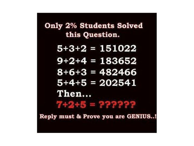
We know there's a correlation between the numbers on the left side, and the answer on the the right side. However, we don't know how they are correlated.
The simplest form for regression is linear regression which you're probably already familiar with. This can be expressed in code like so:
from sklearn.linear_model import LinearRegression

# Dataset
train_X = [[5,3,2],[9,2,4],[8,6,3],[5,4,5]]
train_Y = [151022,183652,482466,202541]

# Create and train model
model = LinearRegression()
model.fit(train_X, train_Y)

print ("5+3+2 = %d" % model.predict([[5,3,2]]))
print ("7+2+5 = %d" % model.predict([[7,2,5]]))

# OUT:
# 5+3+2 = 151022
# 7+2+5 = 107687
Let's examine what happens here?
First, we import the linear regression model from sklearn with from sklearn.linear_model import LinearRegression. Next, we initialize the data; notice how we group the individual features in a list for example [5,3,2] is one set of features for which the label, or the correct answer is the train_Y value at the same index: 151022. We then initialize and train the model using the by now familiar sklearn syntax. Finally, we use the newly fitted model to predict, first one of the known examples to see if it works, and then the unknown test for which we see the answer is 107687.
Validating The Regression Model
Usually in machine learning, you validate the model by segmenting your data into a training set, and a test set. In order to find the generalized accuracy then, you measure the model's accuracy on the test set which ideally contains samples which the model has never seen before. This method usually gives a good indication of how well the model will perform on real world data.
However, for the internet memes, we have so few examples that we have to use everything we have during training. While this is would be a problem if we're trying to fit real world data where noise can occur from outliers, and fallacious measurements, it works for these internet memes due to two important properties.
- All the data is exact. All the inputs
X, when run throughf(x)always equals our valueY. - The function that we are trying to find
f(x)is explicit. That is it does exist, and is not a part of a probability distribution.
This means that we can compute the accuracy from the same data which we use for training, and we know that we have found a correct relationship if and only if the accuracy computed is equal to 1. That is assuming it doesn't memorize the examples.
Why is that? You might ask. The reason we can declare the internet meme correctly solved when the model is 100% accurate is because the meme only asks for a relationship, and not necessarily the same relationship that the original author intended as there's no way of proving what was intended.
So as long as the model is internally consistent all the way through, it can be said to have discovered a true relationship.
But isn't that cheating? You say. To answer this, allow me to pose an example. Suppose I gave you the following numbers [1,2,3,4,5,6,7,8,9,10,11,12], and I asked you to predict the next number based on the pattern. You might say 13, however, that is not the 'correct' solution; it is 1. You, quite reasonably, assumed that I was talking about the natural numbers series, but I was in fact thinking of the hours of the day on a clock where after 12, it loops back to 1.
Does this make your answer incorrect? No, you had every reason to assume I was talking about the natural numbers, and your answer is consistent with the examples I gave you. You cannot be expected to read my mind, so as long as your answer consistent with the examples, it should be regarded as correct. This similarly applies to the internet memes, and the models.
All of this means that we can write code like so:
acc = model.score(train_X, train_Y)

print ("Accuracy: %d" % acc)

# OUT:
# Accuracy: 1
It's seen that the linear regression model does indeed capture a consistent relationship in the data which means that 107687 is a correct solution for the example. It's important, however, to note that there are often multiple correct answers. For this example, 143547 is also a correct answer for instance.
Beyond Linear Regression
Now, to be frank, linear regression is very simple, and I specifically picked this example to be compatible with linear regression. The truth is that most examples are not that easy, so we need more complex models.
Since we don't know anything about the relationship (f(x)) in the meme, it's not unreasonable to just try a bunch of algorithms, and see which ones perform well. Fortunately, this is quite simple, and can be done like so:
# Import a bunch of models
from sklearn.linear_model import LinearRegression
from sklearn.svm import SVR
from sklearn.neighbors import KNeighborsRegressor
from sklearn.tree import DecisionTreeRegressor
from sklearn.ensemble import GradientBoostingRegressor
from sklearn.gaussian_process import GaussianProcessRegressor
from sklearn.cross_decomposition import PLSRegression
from sklearn.ensemble import AdaBoostRegressor

# Add the models to a list
models = [
 LinearRegression(),
 SVR(),
 KNeighborsRegressor(n_neighbors=2),
 DecisionTreeRegressor(),
 GradientBoostingRegressor(),
 GaussianProcessRegressor(),
 PLSRegression(),
 AdaBoostRegressor()
]

# Dataset
train_X = [[5,3,2],[9,2,4],[8,6,3],[5,4,5]]
train_Y = [151022,183652,482466,202541]

# Train each model individually
for model in models:

 model.fit(train_X, train_Y)
 acc = model.score(train_X, train_Y)

 if acc == 1:
   print (model)
   print ("Accuracy: %d" % acc)
   print ("7+2+5 = %d" % model.predict([[7,2,5]]))
You may wonder why I only use one linear algorithm; linear regression, while abstaining from similar algorithms such as stochastic gradient descent (SGD) linear regression. The reason is related to why we don't need to segment the data: Since we know that the function we are trying to predict f(x) is explicit, and that our data is exact, it serves no purpose trying to use a stochastic version that at best can predict the same as a ordinary least squares version (how the LinearRegression model is implemented).
Similarly, we don't use logistic regression as we can assume that the function is continuous in the prediction space. That is the value we are trying to predict in the last example actually exists.
Note further that we have to set n_neighbors to be equal to 2 instead of the default 5 for the k nearest neighbor regressor. This is because the algorithm cannot pick more unique samples than there are total samples for obvious reasons.
By running this, we get the following output:
LinearRegression(copy_X=True, fit_intercept=True, n_jobs=1, normalize=False)
Accuracy: 1
7+2+5 = 107687

DecisionTreeRegressor(criterion='mse', max_depth=None, max_features=None,
          max_leaf_nodes=None, min_impurity_split=1e-07,
          min_samples_leaf=1, min_samples_split=2,
          min_weight_fraction_leaf=0.0, presort=False, random_state=None,
          splitter='best')
Accuracy: 1
7+2+5 = 202541

GaussianProcessRegressor(alpha=1e-10, copy_X_train=True, kernel=None,
            n_restarts_optimizer=0, normalize_y=False,
            optimizer='fmin_l_bfgs_b', random_state=None)
Accuracy: 1
7+2+5 = 18908

AdaBoostRegressor(base_estimator=None, learning_rate=1.0, loss='linear',
        n_estimators=50, random_state=None)
Accuracy: 1
7+2+5 = 202541
We see that there are indeed multiple solutions to the meme that are all internally consistent evident by the accuracy of 1.
Other examples
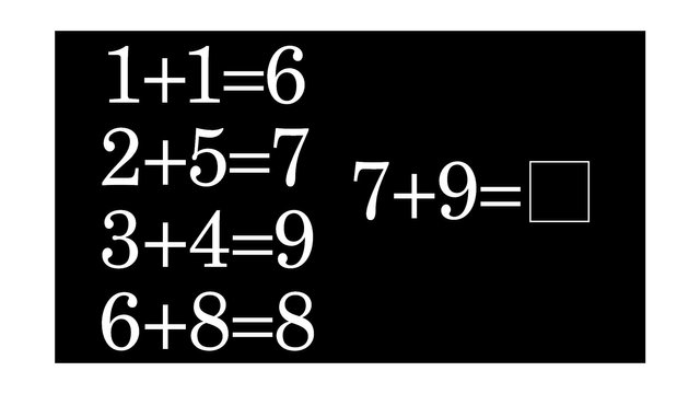
The program would be very limited in its usefulness if it only worked for one example. Running the program for another example is as simple as replacing the data and prediction. Take, for instance, the following meme:

Extracting the data from the image, which we in this tutorial will do by hand, and encoding it into the
# Dataset
train_X = [[5,3],[9,1],[8,6],[5,4]]
train_Y = [28,810,214,19]
pred_X = [7,3]
Notice that we moved the prediction features into the variable pred_X.
Running this, we once again see that there are multiple valid solutions namely 28 and 20.
DecisionTreeRegressor(criterion='mse', max_depth=None, max_features=None,
          max_leaf_nodes=None, min_impurity_split=1e-07,
          min_samples_leaf=1, min_samples_split=2,
          min_weight_fraction_leaf=0.0, presort=False, random_state=None,
          splitter='best')
Accuracy: 1
Prediction: 28

GaussianProcessRegressor(alpha=1e-10, copy_X_train=True, kernel=None,
            n_restarts_optimizer=0, normalize_y=False,
            optimizer='fmin_l_bfgs_b', random_state=None)
Accuracy: 1
Prediction: 20

AdaBoostRegressor(base_estimator=None, learning_rate=1.0, loss='linear',
        n_estimators=50, random_state=None)
Accuracy: 1
Prediction: 28
Tuning the models
The models in sklearn usually comes with sensible default parameters, however, the default parameters are not always the best parameters for the problem. It therefore makes sense to tune the model in order to increase the chance of discovering a consistent pattern. Tuning all the different models manually would be a lot of work.
Sklearn's gridsearch can, well, search through a series of parameters trying different combinations to see which ones have a better accuracy. Gridsearch is also useful in more traditional machine learning problems, but adds a lot of computational overhead as it has to retrain the model every time it a parameter i changed. It can therefore be beneficial to save to best model to disk.
Gridsearch can be implemented like so:
# Import a bunch of models
from sklearn.linear_model import LinearRegression
from sklearn.svm import SVR
from sklearn.neighbors import KNeighborsRegressor
from sklearn.tree import DecisionTreeRegressor
from sklearn.ensemble import GradientBoostingRegressor
from sklearn.gaussian_process import GaussianProcessRegressor
from sklearn.cross_decomposition import PLSRegression
from sklearn.ensemble import AdaBoostRegressor

# Import gridsearch
from sklearn.model_selection import GridSearchCV

# Add the models and grids to a list
models = [
 [LinearRegression(), {"fit_intercept": [True, False]}],
 [SVR(), {"kernel": ["linear", "poly", "rbf", "sigmoid"]}],
 [KNeighborsRegressor(), {"n_neighbors": [1,2], "weights": ["uniform", "distance"]}],
 [DecisionTreeRegressor(), {"criterion": ["mse", "friedman_mse"], "splitter": ["best", "random"],
   "min_samples_split": [x for x in range(2,6)] # generates a list [2,3,4,5]
 }],
 [GradientBoostingRegressor(), {"loss": ["ls", "lad", "huber", "quantile"]}],
 [GaussianProcessRegressor(), {}],
 [PLSRegression(), {}],
 [AdaBoostRegressor(), {}]
]

# Dataset
train_X = [[5,3],[9,1],[8,6],[5,4]]
train_Y = [28,810,214,19]
pred_X = [7,3]

# Train each model individually using grid search
for model in models:
 regressor = model[0]
 param_grid = model[1]

 model = GridSearchCV(regressor, param_grid)
  # Finds the most accurate hyperparameters for the regressor
 # Based on the score function
 model.fit(train_X, train_Y)

 # assess accuracy
 acc = model.score(train_X, train_Y)
  # output model if it's perfect
 if acc == 1:
   print (model)
   print ("Accuracy: %d" % acc)
   print ("Prediction: %d" % model.predict([pred_X]))
   print()
When running this, we get the following output (the parameters are omitted for brevity):
GridSearchCV([...])
Accuracy: 1
Prediction: 23

GridSearchCV([...])
Accuracy: 1
Prediction: 214

GridSearchCV([...])
Accuracy: 1
Prediction: 20

GridSearchCV([...])
Accuracy: 1
Prediction: 28
Conclusion
To recap, we have talked about the differences between classification and regression, and have learned how to use machine learning to solve internet memes.
Finally, we explored one option for automatic optimization.
Homework
- Try to test the program on new examples found on the internet, or examples that we didn't try here.
- Find more relevant features to extend the gridsearch space. Try generating random values.
- Use the techniques you have learned here to solve numeric series such as the fibonacci sequence.
For feedback, send your answers to "homework [at] kasperfred.com". Remember to include the title of the blog post in the subject line.
You can access the entire source code base used in the tutorial here.
Great works, I wish you success
Thanks.